DataInterview

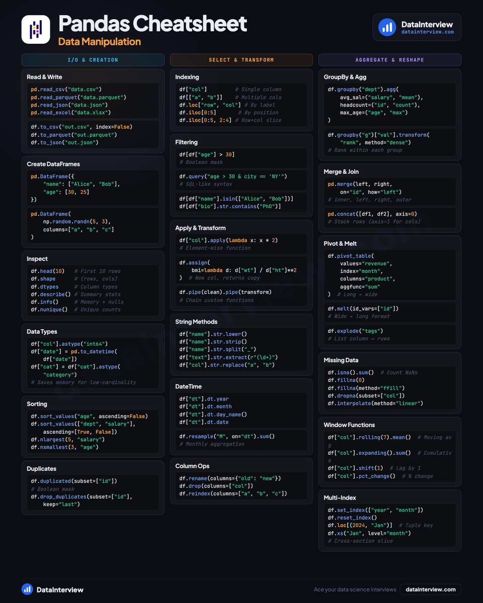
Here's a Pandas cheatsheet for interviews. 👋 Let's explore together ↓ 📥 𝗜/𝗢 & 𝗖𝗿𝗲𝗮𝘁𝗶𝗼𝗻 • Read CSV, Parquet, JSON, Excel • Build DataFrames from dicts or NumPy • Inspect with .shape, .dtypes, .describe() • Cast types, sort values, drop duplicates 🔀 𝗦𝗲𝗹𝗲𝗰𝘁 & 𝗧𝗿𝗮𝗻𝘀𝗳𝗼𝗿𝗺 • loc vs iloc indexing • Boolean masks and .query() filtering • .apply(), .assign(), .pipe() chains • String methods, DateTime accessors • Rename, drop, reindex columns 📊 𝗔𝗴𝗴𝗿𝗲𝗴𝗮𝘁𝗲 & 𝗥𝗲𝘀𝗵𝗮𝗽𝗲 • GroupBy with named agg • Merge, concat, join • Pivot tables and melt • Handle missing data (fillna, interpolate) • Rolling windows and pct_change() • Multi-index slicing with .xs() Save this for your next interview. 👉 Land Data, Quant, AI jobs on datainterview.com

What is the Sharpe Ratio? (in ML interviews) 👋 Let's learn together ↓ 𝗦𝗵𝗮𝗿𝗽𝗲 𝗥𝗮𝘁𝗶𝗼 𝗺𝗲𝗮𝘀𝘂𝗿𝗲𝘀 𝗲𝘅𝗰𝗲𝘀𝘀 𝗿𝗲𝘁𝘂𝗿𝗻 𝗽𝗲𝗿 𝘂𝗻𝗶𝘁 𝗼𝗳 𝗿𝗶𝘀𝗸. It tells you how much extra return you get for taking on volatility. Higher is better. A portfolio with Sharpe = 2 earns twice the excess return per unit of risk compared to one with Sharpe = 1. Think of it as return efficiency. You want the most bang for your buck in risk. 📐 𝗧𝗵𝗲 𝗳𝗼𝗿𝗺𝘂𝗹𝗮: S = (Rp - Rf) / σp Where: Rp → portfolio return Rf → risk-free rate (T-bills, typically) σp → portfolio standard deviation (volatility) The numerator is excess return. The denominator is total risk. ⚡ 𝗛𝗼𝘄 𝘁𝗼 𝗰𝗮𝗹𝗰𝘂𝗹𝗮𝘁𝗲 𝗶𝘁: ① Get your portfolio returns over time ② Subtract the risk-free rate from each return ③ Calculate the mean of those excess returns ④ Calculate the standard deviation of returns ⑤ Divide mean excess return by std dev For daily data, annualize by multiplying by √252 (trading days). 🧐 𝗛𝗼𝘄 𝗶𝘀 𝗶𝘁 𝗱𝗶𝗳𝗳𝗲𝗿𝗲𝗻𝘁 𝗳𝗿𝗼𝗺 𝗦𝗼𝗿𝘁𝗶𝗻𝗼 𝗥𝗮𝘁𝗶𝗼? Sharpe uses total volatility (upside and downside) as the risk measure. It assumes you care equally about all deviations. Sortino only penalizes downside deviation. It ignores upside volatility because big gains aren't really "risk." Sortino is better when returns are asymmetric or you only care about losses. 🎯 𝗜𝗻𝘁𝗲𝗿𝗽𝗿𝗲𝘁𝗶𝗻𝗴 𝘁𝗵𝗲 𝘃𝗮𝗹𝘂𝗲: < 0 → losing money after accounting for risk-free rate 0 to 1 → okay, but not great compensation for risk 1 to 2 → good, strong risk-adjusted returns > 2 → excellent, rare and hard to sustain ✍️ 𝗪𝗵𝗲𝗻 𝘁𝗼 𝘂𝘀𝗲 𝗦𝗵𝗮𝗿𝗽𝗲 𝗥𝗮𝘁𝗶𝗼: when comparing portfolios or strategies with different risk profiles, or when you need a single number to rank investment performance. 👉 Land Data & AI jobs on datainterview.com

What is Correlation vs Causation? (in ML interviews) 👋 Let's learn together ↓ 𝗖𝗼𝗿𝗿𝗲𝗹𝗮𝘁𝗶𝗼𝗻 𝗺𝗲𝗮𝘀𝘂𝗿𝗲𝘀 𝗵𝗼𝘄 𝘁𝘄𝗼 𝘃𝗮𝗿𝗶𝗮𝗯𝗹𝗲𝘀 𝗺𝗼𝘃𝗲 𝘁𝗼𝗴𝗲𝘁𝗵𝗲𝗿. 𝗖𝗮𝘂𝘀𝗮𝘁𝗶𝗼𝗻 𝗺𝗲𝗮𝗻𝘀 𝗼𝗻𝗲 𝗮𝗰𝘁𝘂𝗮𝗹𝗹𝘆 𝗱𝗿𝗶𝘃𝗲𝘀 𝘁𝗵𝗲 𝗼𝘁𝗵𝗲𝗿. Two variables can have perfect correlation (r = 0.98) without any causal link. Ice cream sales and drownings both rise in summer, but neither causes the other. The difference matters. If you intervene on one variable, does the other change? That's the test. 📐 𝗧𝗵𝗲 𝗰𝗼𝗿𝗿𝗲𝗹𝗮𝘁𝗶𝗼𝗻 𝗳𝗼𝗿𝗺𝘂𝗹𝗮: Corr(X,Y) = Cov(X,Y) / (σx × σy) Where: Cov(X,Y) → how X and Y vary together σx, σy → standard deviations Result ranges from -1 to +1 This is symmetric. Corr(X,Y) = Corr(Y,X). No direction implied. 🔍 𝗧𝗵𝗿𝗲𝗲 𝘁𝘆𝗽𝗲𝘀 𝗼𝗳 𝗿𝗲𝗹𝗮𝘁𝗶𝗼𝗻𝘀𝗵𝗶𝗽𝘀: ① 𝗖𝗮𝘂𝘀𝗮𝗹: X directly causes Y (proven via RCT or natural experiment) ② 𝗖𝗼𝗻𝗳𝗼𝘂𝗻𝗱𝗲𝗱: hidden variable Z drives both X and Y (summer heat → ice cream + drowning) ③ 𝗦𝗽𝘂𝗿𝗶𝗼𝘂𝘀: pure coincidence (cheese consumption tracks PhDs, no mechanism) ⚡ 𝗖𝗮𝘂𝘀𝗮𝗹 𝘁𝗵𝗶𝗻𝗸𝗶𝗻𝗴 (𝗣𝗲𝗮𝗿𝗹'𝘀 𝗱𝗼-𝗰𝗮𝗹𝗰𝘂𝗹𝘂𝘀): E[Y | do(X = x)] ≠ E[Y] This asks: if I intervene and set X to x, does Y change? Requires ruling out confounders and reverse causality. Directional, not symmetric. 🧐 𝗞𝗲𝘆 𝗽𝗶𝘁𝗳𝗮𝗹𝗹𝘀 𝘁𝗼 𝘄𝗮𝘁𝗰𝗵: 𝗥𝗲𝘃𝗲𝗿𝘀𝗲 𝗰𝗮𝘂𝘀𝗮𝗹𝗶𝘁𝘆 → maybe Y causes X, not the other way 𝗦𝗶𝗺𝗽𝘀𝗼𝗻'𝘀 𝗽𝗮𝗿𝗮𝗱𝗼𝘅 → trend flips when you split by subgroups 𝗖𝗼𝗻𝗳𝗼𝘂𝗻𝗱𝗲𝗿𝘀 → hidden variables create fake associations 🎯 𝗛𝗼𝘄 𝘁𝗼 𝗲𝘀𝘁𝗮𝗯𝗹𝗶𝘀𝗵 𝗰𝗮𝘂𝘀𝗮𝘁𝗶𝗼𝗻: RCTs → randomize to remove confounders Natural experiments → exploit external shocks DAGs → graph the causal structure Diff-in-diff → compare treated vs control, before/after ✍️ 𝗪𝗵𝗲𝗻 𝘁𝗼 𝘂𝘀𝗲 𝗰𝗮𝘂𝘀𝗮𝗹 𝗿𝗲𝗮𝘀𝗼𝗻𝗶𝗻𝗴: when you need to predict the effect of an intervention, not just observe patterns. Correlation finds signals. Causation tells you what happens when you act. 👉 Land Data & AI jobs on datainterview.com

What is PCA for Returns? (in quant interviews) 👋 Let's learn together ↓ 𝗣𝗖𝗔 𝗳𝗼𝗿 𝗥𝗲𝘁𝘂𝗿𝗻𝘀 decomposes asset return covariance into orthogonal risk factors. Instead of tracking hundreds of correlated stocks, you extract a few independent components that explain most of the variance. PC1 captures market moves, PC2 captures sector tilts, PC3 captures size effects. This turns a messy correlation matrix into clean, interpretable risk drivers. 📐 𝗧𝗵𝗲 𝗱𝗲𝗰𝗼𝗺𝗽𝗼𝘀𝗶𝘁𝗶𝗼𝗻: Σ = W Λ W^T Where: Σ → return covariance matrix W → eigenvectors (factor loadings) Λ → eigenvalues (variance explained per PC) Each return projects as: r_t ≈ sum of w_k f_k,t for k=1 to K 💪 𝗛𝗼𝘄 𝗶𝘁 𝘄𝗼𝗿𝗸𝘀: ① Compute covariance matrix from historical returns ② Solve eigenvalue problem to get W and Λ ③ Sort components by eigenvalue (largest first) ④ Keep top K components that hit your variance threshold (often 70-90%) ⑤ Project returns onto these K factors 🧐 𝗛𝗼𝘄 𝗶𝘀 𝗶𝘁 𝗱𝗶𝗳𝗳𝗲𝗿𝗲𝗻𝘁 𝗳𝗿𝗼𝗺 𝗙𝗮𝗰𝘁𝗼𝗿 𝗠𝗼𝗱𝗲𝗹𝘀? Factor models (Fama-French, Barra) use predefined economic factors like value, momentum, or industry. PCA discovers factors purely from data. No economic labels. PC1 usually ends up being market beta, but PC2 and PC3 are statistical constructs you have to interpret after the fact. Factor models are easier to explain. PCA is more flexible and captures whatever actually drives your returns. ✍️ 𝗪𝗵𝗲𝗻 𝘁𝗼 𝘂𝘀𝗲 𝗣𝗖𝗔 𝗳𝗼𝗿 𝗥𝗲𝘁𝘂𝗿𝗻𝘀: when you need dimensionality reduction for portfolio risk, want to build factor models without economic priors, or need to detect regime changes in correlation structure. 👉 Land Data & AI jobs on datainterview.com

What is Momentum Trading? (in Quant interviews) 👋 Let's learn together ↓ Momentum is a 𝘁𝗿𝗮𝗱𝗶𝗻𝗴 𝘀𝘁𝗿𝗮𝘁𝗲𝗴𝘆 that buys assets trending up and sells assets trending down. The idea: past winners keep winning, past losers keep losing. This persistence happens because investors underreact to news and adjust prices slowly over 6-9 months. You're betting on continuation, not reversal. 📐 𝗧𝗵𝗲 𝘀𝗶𝗴𝗻𝗮𝗹: MOMₜ = (Pₜ / Pₜ₋ₙ) - 1 Where: Pₜ → current price Pₜ₋ₙ → price n periods ago (typically 12 months) MOMₜ → percentage return over lookback window 💪 𝗛𝗼𝘄 𝗶𝘁 𝘄𝗼𝗿𝗸𝘀: ① Calculate returns over lookback period (e.g., 12 months) ② Rank all assets by their momentum score ③ Go long top decile (winners), short bottom decile (losers) ④ Hold for 1 month, then rebalance ⑤ Skip the most recent month to avoid short-term reversals 🧐 𝗛𝗼𝘄 𝗶𝘀 𝗶𝘁 𝗱𝗶𝗳𝗳𝗲𝗿𝗲𝗻𝘁 𝗳𝗿𝗼𝗺 𝗠𝗲𝗮𝗻 𝗥𝗲𝘃𝗲𝗿𝘀𝗶𝗼𝗻? Mean reversion bets prices return to average after moving too far. You buy losers and sell winners. Momentum does the opposite. You buy winners and sell losers, betting the trend continues. Mean reversion works on shorter horizons (days to weeks). Momentum works on medium horizons (3-12 months). They can coexist: prices reverse short-term but trend medium-term. ✍️ 𝗪𝗵𝗲𝗻 𝘁𝗼 𝘂𝘀𝗲 𝗠𝗼𝗺𝗲𝗻𝘁𝘂𝗺: when you believe behavioral persistence drives returns and you can handle sharp crashes during market reversals (like 2009). 👉 Land Data & AI jobs on datainterview.com

What is Monte Carlo Simulation? (in data & quant interviews) 👋 Let’s learn together ↓ Monte Carlo is a 𝗻𝘂𝗺𝗲𝗿𝗶𝗰𝗮𝗹 𝗺𝗲𝗱𝗵𝗼𝗱 that approximates expectations and integrals through repeated random sampling. You draw thousands (or millions) of random samples from a distribution, apply a function to each, then average the results. This gives you an estimate of the true expectation. Works when analytical solutions are impossible or too complex. 📐 𝗧𝗵𝗲 𝗲𝘀𝗱𝗶𝗺𝗮𝗱𝗼𝗿: μ̂ₙ = (1/N) × Σ f(Xᵢ), where Xᵢ ~ p(x) Where: N → number of random samples f(Xᵢ) → function applied to each sample p(x) → target distribution you’re sampling from μ̂ₙ → estimate of E[f(X)] ⚡ 𝗛𝗼𝘀 𝗶𝗱 𝘀𝗼𝗿𝗸𝘀: ① Define the problem as an expectation E[f(X)] ② Draw N independent samples from distribution p(x) ③ Evaluate f(Xᵢ) for each sample ④ Average all results to get your estimate ⑤ Increase N to reduce error 🧐 𝗛𝗼𝘀 𝗶𝘀 𝗶𝗱 𝗱𝗶𝗳𝗳𝗲𝗿𝗲𝗻𝗱 𝗳𝗿𝗼𝗺 𝗻𝘂𝗺𝗲𝗿𝗶𝗰𝗮𝗹 𝗶𝗻𝗱𝗲𝗴𝗿𝗮𝗱𝗶𝗼𝗻? Grid-based methods (like quadrature) evaluate the function at fixed points and struggle in high dimensions. Monte Carlo uses random sampling, so error decreases at rate 1/√N regardless of dimension. This makes it better for problems with many variables. Trade-off: slower convergence but scales to any dimension. ✍️ 𝗪𝗵𝗲𝗻 𝗱𝗼 𝘂𝘀𝗲 𝗠𝗼𝗻𝗱𝗲 𝗖𝗮𝗿𝗹𝗼: when you need to estimate expectations in high dimensions, price options, simulate physical systems, or solve integrals with no closed form. 👉 Land Data & AI jobs on datainterview.com

What is Gradient Descent? (in ML interviews) 👋 Let's learn together ↓ Gradient Descent is an 𝗶𝘁𝗲𝗿𝗮𝘁𝗶𝘃𝗲 𝗼𝗽𝘁𝗶𝗺𝗶𝘇𝗮𝘁𝗶𝗼𝗻 𝗮𝗹𝗴𝗼𝗿𝗶𝘁𝗵𝗺 that finds the minimum of a loss function. It works by repeatedly taking steps in the direction opposite to the gradient. Think of it like walking downhill in fog. You can't see the bottom, but you can feel which way is steepest and move that direction. The gradient points uphill (steepest ascent), so we subtract it to go downhill. 📐 𝗧𝗵𝗲 𝘂𝗽𝗱𝗮𝘁𝗲 𝗿𝘂𝗹𝗲: θₜ₊₁ = θₜ - α∇J(θₜ) Where: θₜ → current parameters α → learning rate (step size) ∇J(θₜ) → gradient of loss function at current position ⚡ 𝗛𝗼𝘄 𝗶𝘁 𝘄𝗼𝗿𝗸𝘀: ① Start with random parameter values ② Compute gradient of loss with respect to parameters ③ Update parameters by moving opposite to gradient ④ Repeat until loss stops decreasing (convergence) The learning rate controls how big each step is. Too large and you overshoot the minimum. Too small and training takes forever. 🔍 𝗛𝗼𝘄 𝗶𝘀 𝗶𝘁 𝗱𝗶𝗳𝗳𝗲𝗿𝗲𝗻𝘁 𝗳𝗿𝗼𝗺 𝗦𝘁𝗼𝗰𝗵𝗮𝘀𝘁𝗶𝗰 𝗚𝗗? Batch GD uses all N samples per update. Stable but slow. Stochastic GD uses one random sample per update. Noisy but fast. Mini-batch GD uses 32-512 samples. Best of both worlds and the default in practice. ✍️ 𝗪𝗵𝗲𝗻 𝘁𝗼 𝘂𝘀𝗲 𝗚𝗿𝗮𝗱𝗶𝗲𝗻𝘁 𝗗𝗲𝘀𝗰𝗲𝗻𝘁: when you need to minimize a differentiable loss function and can compute gradients. It's the foundation of training neural networks. 👉 Land Data & AI jobs on datainterview.com

What is Survival Analysis? (in data & quant interviews) 👋 Let's learn together ↓ Survival analysis models 𝘁𝗶𝗺𝗲-𝘁𝗼-𝗲𝘃𝗲𝗻𝘁 𝗱𝗮𝘁𝗮 with censoring. It predicts when events happen, not just whether they will. The event could be death, churn, machine failure, or loan default. The key challenge: some observations are censored (we don't see the event yet). This makes standard regression fail. You need methods that handle incomplete information. 📐 𝗧𝗵𝗲 𝗰𝗼𝗿𝗲 𝗳𝘂𝗻𝗰𝘁𝗶𝗼𝗻𝘀: S(t) = P(T > t) = e^(-∫h(u)du) Where: S(t) → survival function (probability of surviving past time t) h(t) → hazard function (instantaneous failure rate at time t) T → time until event The hazard tells you risk at each moment. The survival function tells you cumulative probability of making it past t. 💪 𝗞𝗮𝗽𝗹𝗮𝗻-𝗠𝗲𝗶𝗲𝗿 𝗲𝘀𝘁𝗶𝗺𝗮𝘁𝗼𝗿 (𝗻𝗼𝗻-𝗽𝗮𝗿𝗮𝗺𝗲𝘁𝗿𝗶𝗰): S(t) = product of (1 - di/ni) for all event times ≤ t Where: di → number of events at time i ni → number at risk just before time i ① Sort event times ② At each event time, calculate proportion surviving ③ Multiply survival proportions together ④ Result: step function dropping at each event Handles right-censored data naturally by adjusting the risk set. ⚡ 𝗖𝗼𝘅 𝗣𝗿𝗼𝗽𝗼𝗿𝘁𝗶𝗼𝗻𝗮𝗹 𝗛𝗮𝘇𝗮𝗿𝗱𝘀 (𝘀𝗲𝗺𝗶-𝗽𝗮𝗿𝗮𝗺𝗲𝘁𝗿𝗶𝗰): h(t|X) = h0(t) × e^(β'X) Where: h0(t) → baseline hazard (unspecified) β'X → linear combination of covariates Key assumption: hazard ratios are constant over time. If someone has twice the risk at t=1, they have twice the risk at t=10. You don't estimate h0(t) directly. You estimate β coefficients via partial likelihood. 🧐 𝗛𝗼𝘄 𝗶𝘀 𝗶𝘁 𝗱𝗶𝗳𝗳𝗲𝗿𝗲𝗻𝘁 𝗳𝗿𝗼𝗺 𝗹𝗼𝗴𝗶𝘀𝘁𝗶𝗰 𝗿𝗲𝗴𝗿𝗲𝘀𝘀𝗶𝗼𝗻? Logistic regression predicts binary outcomes (event yes/no) and ignores timing. It can't handle censoring properly. Survival analysis predicts when events occur and uses all available information from censored cases. It models the time dimension explicitly. Cox models also give you hazard ratios, which are easier to interpret than odds ratios for time-varying risk. 🎯 𝗖𝗼𝗺𝗺𝗼𝗻 𝗲𝘃𝗮𝗹𝘂𝗮𝘁𝗶𝗼𝗻 𝗺𝗲𝘁𝗿𝗶𝗰𝘀: C-index → concordance between predicted risk and observed order (like AUC for survival). 1.0 is perfect, 0.5 is random. Log-rank test → compares survival curves between groups. Tests if two Kaplan-Meier curves differ significantly. Brier score → time-dependent prediction accuracy combining calibration and discrimination. ✍️ 𝗪𝗵𝗲𝗻 𝘁𝗼 𝘂𝘀𝗲 𝘀𝘂𝗿𝘃𝗶𝘃𝗮𝗹 𝗮𝗻𝗮𝗹𝘆𝘀𝗶𝘀: when you care about time until an event and have censored observations (customer churn, patient survival, equipment failure, loan default). 👉 Land Data & AI jobs on datainterview.com

What is Bayes' Theorem? (in ML interviews) 👋 Let's learn together ↓ 𝗕𝗮𝘆𝗲𝘀' 𝗧𝗵𝗲𝗼𝗿𝗲𝗺 𝗶𝘀 𝗮 𝗳𝗼𝗿𝗺𝘂𝗹𝗮 𝗳𝗼𝗿 𝘂𝗽𝗱𝗮𝘁𝗶𝗻𝗴 𝗯𝗲𝗹𝗶𝗲𝗳𝘀 𝘄𝗶𝘁𝗵 𝗲𝘃𝗶𝗱𝗲𝗻𝗰𝗲. It tells you how to revise your initial belief (prior) after seeing new data. This is the foundation of probabilistic reasoning in machine learning. You start with what you know, observe evidence, and calculate an updated belief (posterior). 📐 𝗧𝗵𝗲 𝗳𝗼𝗿𝗺𝘂𝗹𝗮: P(A | B) = P(B | A) × P(A) / P(B) Where: P(A | B) → posterior (updated belief after seeing B) P(B | A) → likelihood (probability of evidence given hypothesis) P(A) → prior (initial belief before evidence) P(B) → marginal evidence (total probability of observing B) The denominator normalizes so probabilities sum to 1 across all hypotheses. ⚡ 𝗛𝗼𝘄 𝗶𝘁 𝘄𝗼𝗿𝗸𝘀 (𝗺𝗲𝗱𝗶𝗰𝗮𝗹 𝘁𝗲𝘀𝘁 𝗲𝘅𝗮𝗺𝗽𝗹𝗲): ① Disease prevalence is 1% (prior) ② Test has 90% sensitivity and 5% false positive rate (likelihoods) ③ You test positive ④ Apply Bayes: P(sick | positive) = (0.90 × 0.01) / (0.90 × 0.01 + 0.05 × 0.99) ⑤ Result: only 15.4% chance you are actually sick Most positive tests are false alarms when the disease is rare. The base rate matters more than you think. 🎯 𝗣𝗼𝘀𝘁𝗲𝗿𝗶𝗼𝗿 𝗼𝗱𝗱𝘀 𝗳𝗼𝗿𝗺 (𝘂𝘀𝗲𝗳𝘂𝗹 𝗳𝗼𝗿 𝘀𝗲𝗾𝘂𝗲𝗻𝘁𝗶𝗮𝗹 𝘂𝗽𝗱𝗮𝘁𝗲𝘀): P(A|B) / P(¬A|B) = [P(B|A) / P(B|¬A)] × [P(A) / P(¬A)] This separates the update signal (likelihood ratio) from your prior belief (prior odds). Makes sequential updates cleaner. 🧐 𝗛𝗼𝘄 𝗶𝘀 𝗶𝘁 𝗱𝗶𝗳𝗳𝗲𝗿𝗲𝗻𝘁 𝗳𝗿𝗼𝗺 𝗳𝗿𝗲𝗾𝘂𝗲𝗻𝘁𝗶𝘀𝘁 𝗶𝗻𝗳𝗲𝗿𝗲𝗻𝗰𝗲? Frequentist methods treat parameters as fixed unknowns and use p-values. No prior beliefs allowed. Bayesian methods treat parameters as random variables with distributions. You start with a prior, update with data, and get a posterior distribution over possible values. Bayesian gives you probability statements about parameters. Frequentist gives you long-run error rates. 💪 𝗞𝗲𝘆 𝗮𝘀𝘀𝘂𝗺𝗽𝘁𝗶𝗼𝗻𝘀: You need a prior (subjective or empirical). Events must be exhaustive and mutually exclusive. Naive Bayes assumes conditional independence of features given the class (rarely true, but works anyway). 🔍 𝗣𝗿𝗮𝗰𝘁𝗶𝗰𝗮𝗹 𝘁𝗶𝗽𝘀: Use log-odds to avoid numerical underflow with many features. Conjugate priors (like Beta for Bernoulli) make posterior updates analytically tractable. Always account for base rates or you will overweight the likelihood. ✍️ 𝗪𝗵𝗲𝗻 𝘁𝗼 𝘂𝘀𝗲 𝗕𝗮𝘆𝗲𝘀' 𝗧𝗵𝗲𝗼𝗿𝗲𝗺: for Naive Bayes classifiers (text, spam filtering), Bayesian optimization (hyperparameter tuning), and Bayesian neural networks (uncertainty estimation). Anytime you want to quantify uncertainty or update beliefs with new data. 👉 Land Data & AI jobs on datainterview.com

What is the Beta Distribution? (in data & quant interviews) 👋 Let's learn together ↓ The Beta Distribution is a 𝗳𝗹𝗲𝘅𝗶𝗯𝗹𝗲 𝗽𝗿𝗼𝗯𝗮𝗯𝗶𝗹𝗶𝘁𝘆 𝗱𝗶𝘀𝘁𝗿𝗶𝗯𝘂𝘁𝗶𝗼𝗻 𝗳𝗼𝗿 𝘃𝗮𝗹𝘂𝗲𝘀 𝗯𝗲𝘁𝘄𝗲𝗲𝗻 𝟬 𝗮𝗻𝗱 𝟭. It models probabilities themselves. Think conversion rates, click-through rates, or success proportions. Two shape parameters (α and β) control whether the distribution peaks near 0, near 1, or somewhere in between. It's the go-to distribution when you need to represent uncertainty about a probability. 📐 𝗧𝗵𝗲 𝗳𝗼𝗿𝗺𝘂𝗹𝗮: f(x; α, β) = [x^(α-1) × (1-x)^(β-1)] / B(α, β) Where: x → value between 0 and 1 α → shape parameter (pseudo-count of successes) β → shape parameter (pseudo-count of failures) B(α, β) → Beta function normalizing constant ⚡ 𝗛𝗼𝘄 𝘁𝗵𝗲 𝗽𝗮𝗿𝗮𝗺𝗲𝘁𝗲𝗿𝘀 𝘄𝗼𝗿𝗸: ① α = β = 1 gives you a uniform distribution (flat line) ② α > β pushes density toward 1 (more successes) ③ β > α pushes density toward 0 (more failures) ④ Larger α + β makes the distribution tighter (more confident) 🎯 𝗛𝗼𝘄 𝗶𝘀 𝗶𝘁 𝗱𝗶𝗳𝗳𝗲𝗿𝗲𝗻𝘁 𝗳𝗿𝗼𝗺 𝘁𝗵𝗲 𝗕𝗶𝗻𝗼𝗺𝗶𝗮𝗹? Binomial models the number of successes in n trials (discrete outcomes). Beta models the probability of success itself (continuous between 0 and 1). Beta is actually the conjugate prior for the Binomial. After observing data, your posterior is still Beta with updated parameters. ✍️ 𝗪𝗵𝗲𝗻 𝘁𝗼 𝘂𝘀𝗲 𝗕𝗲𝘁𝗮: when you need to model uncertainty about a rate, proportion, or probability. Common in Bayesian A/B testing, conversion rate estimation, and Thompson Sampling for bandits. 👉 Land Data & AI jobs on datainterview.com

What is GARCH Modeling? (in Quant interviews) 👋 Let's learn together ↓ GARCH is a 𝘁𝗶𝗺𝗲 𝘀𝗲𝗿𝗶𝗲𝘀 𝗺𝗼𝗱𝗲𝗹 𝗳𝗼𝗿 𝘃𝗼𝗹𝗮𝘁𝗶𝗹𝗶𝘁𝘆 𝗰𝗹𝘂𝘀𝘁𝗲𝗿𝗶𝗻𝗴. It captures how variance changes over time in financial returns. Big shocks create periods of high volatility that persist, then slowly decay back to normal. Think: market turbulence after a crash, where wild swings cluster together before calming down. 📐 𝗧𝗵𝗲 𝗺𝗼𝗱𝗲𝗹 (𝗚𝗔𝗥𝗖𝗛(𝟭,𝟭)): σ²ₜ = ω + α·ε²ₜ₋₁ + β·σ²ₜ₋₁ Where: σ²ₜ → conditional variance at time t ω → long-run baseline variance α → ARCH term (impact of past shocks) ε²ₜ₋₁ → squared residual from previous period β → GARCH term (persistence of past volatility) ⚡ 𝗛𝗼𝘄 𝗶𝘁 𝘄𝗼𝗿𝗸𝘀: ① Start with a mean model for returns (like ARMA) ② Extract residuals (shocks) ③ Model variance of residuals using past shocks and past variance ④ Estimate parameters via maximum likelihood ⑤ Forecast future volatility using the fitted model High α means shocks hit hard. High β means volatility sticks around. Their sum (α+β) measures persistence. Close to 1 means volatility decays slowly. 🧐 𝗛𝗼𝘄 𝗶𝘀 𝗶𝘁 𝗱𝗶𝗳𝗳𝗲𝗿𝗲𝗻𝘁 𝗳𝗿𝗼𝗺 𝗔𝗥𝗖𝗛? ARCH only uses past shocks (ε²ₜ₋₁, ε²ₜ₋₂, ...) to model variance. You need many lags to capture persistence. GARCH adds past variance (σ²ₜ₋₁) as a predictor. This creates a more compact model with fewer parameters that still captures long memory in volatility. ARCH(p) with many lags becomes GARCH(1,1) with just three parameters. ✍️ 𝗪𝗵𝗲𝗻 𝘁𝗼 𝘂𝘀𝗲 𝗚𝗔𝗥𝗖𝗛: when modeling financial returns, risk management, or any time series where variance isn't constant and shocks create persistent volatility clusters. 👉 Land Data & AI jobs on datainterview.com

What is Modern Portfolio Theory? (in quant interviews) 👋 Let's learn together ↓ 𝗠𝗣𝗧 𝗶𝘀 𝗮 𝗳𝗿𝗮𝗺𝗲𝘄𝗼𝗿𝗸 𝗳𝗼𝗿 𝗯𝘂𝗶𝗹𝗱𝗶𝗻𝗴 𝗽𝗼𝗿𝘁𝗳𝗼𝗹𝗶𝗼𝘀 𝘁𝗵𝗮𝘁 𝗺𝗮𝘅𝗶𝗺𝗶𝘇𝗲 𝗿𝗲𝘁𝘂𝗿𝗻 𝗳𝗼𝗿 𝗮 𝗴𝗶𝘃𝗲𝗻 𝗿𝗶𝘀𝗸 𝗹𝗲𝘃𝗲𝗹. The big idea: diversification works because assets don't move in lockstep. By combining low-correlation assets, you reduce total portfolio risk without sacrificing returns. This is the foundation of quantitative finance. Harry Markowitz won a Nobel Prize for it. 📐 𝗧𝗵𝗲 𝗺𝗮𝘁𝗵: Minimize: wᵀΣw Subject to: wᵀμ = μₚ, wᵀ1 = 1 Where: w → vector of asset weights Σ → covariance matrix (captures correlations) μ → expected returns vector μₚ → target portfolio return Portfolio variance: σₚ² = ΣᵢΣⱼ wᵢwⱼσᵢⱼ The key insight: total risk depends on pairwise covariances, not just individual variances. ⚡ 𝗛𝗼𝘄 𝗶𝘁 𝘄𝗼𝗿𝗸𝘀: ① Define your universe of assets with expected returns and covariances ② Pick a target return level ③ Solve the quadratic optimization to find weights that minimize variance ④ Repeat for different target returns to trace out the efficient frontier ⑤ Select the tangency portfolio (max Sharpe ratio) for optimal risk-adjusted returns The efficient frontier shows all portfolios with maximum return for each risk level. 🧐 𝗛𝗼𝘄 𝗶𝘀 𝗶𝘁 𝗱𝗶𝗳𝗳𝗲𝗿𝗲𝗻𝘁 𝗳𝗿𝗼𝗺 𝗕𝗹𝗮𝗰𝗸-𝗟𝗶𝘁𝘁𝗲𝗿𝗺𝗮𝗻? MPT finds optimal portfolios given expected returns and covariances you provide. Black-Litterman starts with market equilibrium returns and lets you blend in your own views. It's Bayesian. You get more stable, less extreme weights because it doesn't rely entirely on your estimates. MPT is the foundation. Black-Litterman fixes its garbage-in-garbage-out problem. ✍️ 𝗪𝗵𝗲𝗻 𝘁𝗼 𝘂𝘀𝗲 𝗠𝗣𝗧: when you need a systematic way to balance risk and return across multiple assets, or when explaining why diversification mathematically reduces risk. 👉 Land Data & AI jobs on datainterview.com

What is the Exponential Distribution? (in data & quant interviews) 👋 Let's learn together ↓ The exponential distribution is a 𝗰𝗼𝗻𝘁𝗶𝗻𝘂𝗼𝘂𝘀 𝗽𝗿𝗼𝗯𝗮𝗯𝗶𝗹𝗶𝘁𝘆 𝗱𝗶𝘀𝘁𝗿𝗶𝗯𝘂𝘁𝗶𝗼𝗻 that models waiting times between independent events. It answers: how long until the next event happens? If customers arrive at rate λ = 3 per hour, how long until the next customer shows up? That wait time follows an exponential distribution. The key insight: it's memoryless. Past waiting gives no information about future waiting. 📐 𝗧𝗵𝗲 𝗺𝗼𝗱𝗲𝗹: f(x) = λe^(-λx) for x ≥ 0 Where: λ → rate parameter (events per unit time) x → time until next event e^(-λx) → exponential decay term The CDF (probability event occurs by time x): F(x) = 1 - e^(-λx) ⚡ 𝗞𝗲𝘆 𝗽𝗿𝗼𝗽𝗲𝗿𝘁𝗶𝗲𝘀: ① Mean = 1/λ (average wait time) ② Variance = 1/λ² (spread of wait times) ③ Median = ln(2)/λ (50th percentile) ④ Mode = 0 (most likely time is right now) ⑤ Memoryless: P(X > s+t | X > s) = P(X > t) The memoryless property means if you've already waited 10 minutes, the probability of waiting another 5 minutes is the same as if you just started. 🧐 𝗛𝗼𝘄 𝗶𝘀 𝗶𝘁 𝗱𝗶𝗳𝗳𝗲𝗿𝗲𝗻𝘁 𝗳𝗿𝗼𝗺 𝗣𝗼𝗶𝘀𝘀𝗼𝗻? Poisson counts how many events happen in a fixed time window (discrete). Exponential measures how long until the next event (continuous). They're connected: if event counts follow Poisson(λ), then time between events follows Exponential(λ). Same rate parameter, different questions. ✍️ 𝗪𝗵𝗲𝗻 𝘁𝗼 𝘂𝘀𝗲 𝗘𝘅𝗽𝗼𝗻𝗲𝗻𝘁𝗶𝗮𝗹: when modeling customer arrival times, component failure times, or any process where events happen independently at a constant average rate. 👉 Land Data & AI jobs on datainterview.com

What is the Bias-Variance Tradeoff? (in ML interviews) 👋 Let's learn together ↓ The bias-variance tradeoff is the 𝗳𝘂𝗻𝗱𝗮𝗺𝗲𝗻𝘁𝗮𝗹 𝗱𝗲𝗰𝗼𝗺𝗽𝗼𝘀𝗶𝘁𝗶𝗼𝗻 𝗼𝗳 𝗽𝗿𝗲𝗱𝗶𝗰𝘁𝗶𝗼𝗻 𝗲𝗿𝗿𝗼𝗿. Every model's error splits into three parts: squared bias, variance, and noise. You can't minimize both bias and variance at once. Reducing one typically increases the other. This is why model selection matters. 📐 𝗧𝗵𝗲 𝗱𝗲𝗰𝗼𝗺𝗽𝗼𝘀𝗶𝘁𝗶𝗼𝗻: MSE = Bias²(f̂) + Var(f̂) + σ² Where: Bias²(f̂) → squared difference between average prediction and truth Var(f̂) → how much predictions vary across different training sets σ² → irreducible noise (data randomness you can't eliminate) 🧮 𝗪𝗵𝗮𝘁 𝗲𝗮𝗰𝗵 𝗰𝗼𝗺𝗽𝗼𝗻𝗲𝗻𝘁 𝗺𝗲𝗮𝗻𝘀: ① 𝗛𝗶𝗴𝗵 𝗯𝗶𝗮𝘀: model is too simple and underfits. It consistently misses the true pattern. ② 𝗛𝗶𝗴𝗵 𝘃𝗮𝗿𝗶𝗮𝗻𝗰𝗲: model is too complex and overfits. Predictions swing wildly with different training data. ③ 𝗦𝘄𝗲𝗲𝘁 𝘀𝗽𝗼𝘁: balanced model minimizes total error by accepting some bias and some variance. ④ 𝗡𝗼𝗶𝘀𝗲: always present. No model can reduce it. ⚡ 𝗛𝗼𝘄 𝗶𝘁 𝗴𝘂𝗶𝗱𝗲𝘀 𝗺𝗼𝗱𝗲𝗹 𝘀𝗲𝗹𝗲𝗰𝘁𝗶𝗼𝗻: Simple models (linear regression on nonlinear data) have high bias, low variance. They underfit. Complex models (deep trees, k-NN with k=1) have low bias, high variance. They overfit. The goal is finding the complexity level where total error bottoms out. Cross-validation helps you estimate this sweet spot without seeing test data. Regularization (L1/L2) lets you reduce variance by adding controlled bias. ✍️ 𝗪𝗵𝗲𝗻 𝘁𝗼 𝘂𝘀𝗲 𝘁𝗵𝗶𝘀 𝗳𝗿𝗮𝗺𝗲𝘄𝗼𝗿𝗸: when choosing between models, tuning complexity, or explaining why your fancy neural net performs worse than a simple baseline on small data. 👉 Land Data & AI jobs on datainterview.com

What is the Normal Distribution? (in ML interviews) 👋 Let's learn together ↓ The normal distribution is a 𝗰𝗼𝗻𝘁𝗶𝗻𝘂𝗼𝘂𝘀 𝗽𝗿𝗼𝗯𝗮𝗯𝗶𝗹𝗶𝘁𝘆 𝗱𝗶𝘀𝘁𝗿𝗶𝗯𝘂𝘁𝗶𝗼𝗻 that forms a symmetric bell curve. It's the most important distribution in statistics and ML. Shows up everywhere: CLT, hypothesis testing, confidence intervals, feature distributions, weight initialization. Fully defined by just two parameters. That's it. 📐 𝗧𝗵𝗲 𝗳𝗼𝗿𝗺𝘂𝗹𝗮: f(x) = (1 / σ√2π) × e^(-½((x-μ)/σ)²) Where: μ → mean (center of the curve) σ → standard deviation (controls spread) σ² → variance 🧮 𝗞𝗲𝘆 𝗽𝗿𝗼𝗽𝗲𝗿𝘁𝗶𝗲𝘀: ① Mean = Median = Mode (perfect symmetry) ② 68% of data within 1σ, 95% within 2σ, 99.7% within 3σ ③ Skewness = 0, Kurtosis = 3 ④ Sum of independent normals is also normal ⑤ Tails extend to infinity but probability drops fast ⚡ 𝗭-𝘀𝗰𝗼𝗿𝗲 𝘀𝘁𝗮𝗻𝗱𝗮𝗿𝗱𝗶𝘇𝗮𝘁𝗶𝗼𝗻: Z = (X - μ) / σ Transforms any normal variable into the standard normal N(0,1). Lets you look up probabilities in Z-tables. Critical for hypothesis testing and comparing values across different scales. 🔍 𝗛𝗼𝘄 𝗶𝘀 𝗶𝘁 𝗱𝗶𝗳𝗳𝗲𝗿𝗲𝗻𝘁 𝗳𝗿𝗼𝗺 𝘁𝗵𝗲 𝘁-𝗱𝗶𝘀𝘁𝗿𝗶𝗯𝘂𝘁𝗶𝗼𝗻? Normal assumes you know σ and works for any sample size. t-distribution is for when σ is unknown (estimated from data) and has heavier tails for small samples (n < 30). As n grows, t converges to normal. ✍️ 𝗪𝗵𝗲𝗻 𝘁𝗼 𝘂𝘀𝗲 𝘁𝗵𝗲 𝗡𝗼𝗿𝗺𝗮𝗹 𝗗𝗶𝘀𝘁𝗿𝗶𝗯𝘂𝘁𝗶𝗼𝗻: when modeling naturally occurring phenomena, applying CLT with large samples, initializing neural network weights, or assuming feature distributions in Naive Bayes. 👉 Land Data & AI jobs on datainterview.com

What is the Chi-Square Distribution? (in data & quant interviews) 👋 Let's learn together ↓ The chi-square distribution is a 𝗽𝗿𝗼𝗯𝗮𝗯𝗶𝗹𝗶𝘁𝘆 𝗱𝗶𝘀𝘁𝗿𝗶𝗯𝘂𝘁𝗶𝗼𝗻 for sums of squared standard normal variables. It's the foundation for hypothesis testing with categorical data. When you test independence between two variables or check if observed counts match expected counts, you're using this distribution. The shape depends entirely on degrees of freedom (k). Low k gives a right-skewed curve. High k looks more normal. 📐 𝗧𝗵𝗲 𝗺𝗮𝘁𝗵: f(x; k) = (x^(k/2-1) × e^(-x/2)) / (2^(k/2) × Γ(k/2)) Where: x → the chi-square statistic (always ≥ 0) k → degrees of freedom Γ → gamma function (generalizes factorials) 🧮 𝗛𝗼𝘄 𝗶𝘁'𝘀 𝗰𝗼𝗻𝘀𝘁𝗿𝘂𝗰𝘁𝗲𝗱: ① Take k independent standard normal variables Z₁, Z₂, ..., Zₖ ② Square each one ③ Add them up: χ² = Z₁² + Z₂² + ... + Zₖ² ④ This sum follows a chi-square distribution with k degrees of freedom Properties: mean = k, variance = 2k, always positive, right-skewed. 🔍 𝗛𝗼𝘄 𝗶𝘀 𝗶𝘁 𝗱𝗶𝗳𝗳𝗲𝗿𝗲𝗻𝘁 𝗳𝗿𝗼𝗺 𝘁𝗵𝗲 𝗡𝗼𝗿𝗺𝗮𝗹 𝗗𝗶𝘀𝘁𝗿𝗶𝗯𝘂𝘁𝗶𝗼𝗻? Normal is symmetric and ranges from negative to positive infinity. Used for continuous measurements. Chi-square is right-skewed, only positive values, and built from squared normals. Used for testing fit and independence in count data. As k increases, chi-square approaches normal shape but never goes negative. ✍️ 𝗪𝗵𝗲𝗻 𝘁𝗼 𝘂𝘀𝗲 𝗖𝗵𝗶-𝗦𝗾𝘂𝗮𝗿𝗲: testing if observed frequencies match expected ones, checking independence in contingency tables, or validating if sample variance matches population variance. 👉 Land Data & AI jobs on datainterview.com

What is the Geometric Distribution? (in data & quant interviews) 👋 Let’s learn together ↓ The geometric distribution models 𝗱𝗵𝗲 𝗻𝘂𝗺𝗯𝗲𝗿 𝗼𝗳 𝗶𝗻𝗱𝗲𝗽𝗲𝗻𝗱𝗲𝗻𝗱 𝗱𝗿𝗶𝗮𝗹𝘀 𝘂𝗻𝗱𝗶𝗹 𝗱𝗵𝗲 𝗳𝗶𝗿𝘀𝗱 𝘀𝘂𝗰𝗰𝗲𝘀𝘀. Think flipping a coin until you get heads. Or calling customers until someone buys. Each trial is independent with the same success probability p. The distribution tells you how likely it is to wait exactly k trials before succeeding. 📐 𝗧𝗵𝗲 𝗳𝗼𝗿𝗺𝘂𝗹𝗮: P(X = k) = (1 - p)^(k-1) × p for k = 1, 2, 3, ... Where: p → probability of success on each trial k → trial number where first success occurs (1 - p)^(k-1) → probability of k-1 failures before success Expected value: E[X] = 1/p Variance: Var(X) = (1-p)/p² ⚡ 𝗛𝗼𝘀 𝗶𝗱 𝘀𝗼𝗿𝗸𝘀: ① Each trial is a Bernoulli experiment (success or failure) ② Trials are independent (past failures don’t change future odds) ③ Success probability p stays constant ④ Count stops at the first success ⑤ Support is unbounded (k can be any positive integer) 🧐 𝗛𝗼𝘀 𝗶𝘀 𝗶𝗱 𝗱𝗶𝗳𝗳𝗲𝗿𝗲𝗻𝗱 𝗳𝗿𝗼𝗺 𝗕𝗶𝗻𝗼𝗺𝗶𝗮𝗹? Geometric counts trials until the first success. Support is unbounded (1, 2, 3, ...). You don’t know when you’ll stop. Binomial counts successes in a fixed number of trials. Support is bounded (0 to n). You know exactly how many trials you’ll run. Both use independent Bernoulli trials with parameter p, but they answer different questions. ✍️ 𝗪𝗵𝗲𝗻 𝗱𝗼 𝘂𝘀𝗲 𝗚𝗲𝗼𝗺𝗲𝗱𝗿𝗶𝗰: when you’re modeling waiting time or number of attempts until something happens for the first time. 👉 Land Data & AI jobs on datainterview.com

What is the Kelly Criterion? (in data & quant interviews) 👋 Let's learn together ↓ The Kelly Criterion is a 𝗯𝗲𝘁 𝘀𝗶𝘇𝗶𝗻𝗴 𝗳𝗼𝗿𝗺𝘂𝗹𝗮 that tells you what fraction of your bankroll to wager to maximize long-term growth. It balances greed and safety. Bet too much and you risk ruin. Bet too little and you leave money on the table. Kelly finds the sweet spot where your wealth compounds fastest over time. 📐 𝗧𝗵𝗲 𝗳𝗼𝗿𝗺𝘂𝗹𝗮: f* = (bp - q) / b Where: f* → optimal fraction of bankroll to wager p → probability of winning q → probability of losing (1 - p) b → net odds (payout per $1 risked) ⚡ 𝗛𝗼𝘄 𝗶𝘁 𝘄𝗼𝗿𝗸𝘀: ① Calculate your edge: bp - q ② Divide by the odds b ③ Result is the fraction to bet ④ If f* ≤ 0, don't bet (no edge) The formula maximizes the expected logarithm of wealth, which is the same as maximizing geometric growth rate. This ensures optimal compounding. 🧐 𝗛𝗼𝘄 𝗶𝘀 𝗶𝘁 𝗱𝗶𝗳𝗳𝗲𝗿𝗲𝗻𝘁 𝗳𝗿𝗼𝗺 𝗳𝗶𝘅𝗲𝗱 𝗯𝗲𝘁𝘁𝗶𝗻𝗴? Fixed betting uses the same dollar amount every time, regardless of edge or bankroll size. Kelly scales with your bankroll and adjusts for the strength of your edge. It grows faster when you're winning and protects you from ruin when losing. Fixed betting ignores compounding. Kelly exploits it. Over-betting (more than Kelly) creates massive drawdown risk. Under-betting (fractional Kelly like ½ or ¼) reduces variance but grows slower. ✍️ 𝗪𝗵𝗲𝗻 𝘁𝗼 𝘂𝘀𝗲 𝗞𝗲𝗹𝗹𝘆: when you have a known edge, can estimate probabilities accurately, and want to maximize long-term growth without going broke. 👉 Land Data & AI jobs on datainterview.com

What are The Greeks? (in Quant interviews) 👋 Let's learn together ↓ 𝗧𝗵𝗲 𝗚𝗿𝗲𝗲𝗸𝘀 𝗮𝗿𝗲 𝗽𝗮𝗿𝘁𝗶𝗮𝗹 𝗱𝗲𝗿𝗶𝘃𝗮𝘁𝗶𝘃𝗲𝘀 𝘁𝗵𝗮𝘁 𝗺𝗲𝗮𝘀𝘂𝗿𝗲 𝗼𝗽𝘁𝗶𝗼𝗻 𝗽𝗿𝗶𝗰𝗲 𝘀𝗲𝗻𝘀𝗶𝘁𝗶𝘃𝗶𝘁𝘆. They tell you how an option's value changes when market conditions shift. Stock moves up? Delta tells you the impact. Time passes? Theta shows the decay. Each Greek isolates one risk factor while holding others constant. 📐 𝗧𝗵𝗲 𝗺𝗮𝗶𝗻 𝗚𝗿𝗲𝗲𝗸𝘀: Delta (Δ) = ∂C/∂S → rate of change w.r.t. stock price → ranges from 0 to 1 for calls, -1 to 0 for puts → approximates probability of expiring ITM Gamma (Γ) = ∂²C/∂S² = ∂Δ/∂S → rate of change of Delta → highest for ATM options near expiry Theta (Θ) = ∂C/∂t → time decay per day → always negative for long options Vega (ν) = ∂C/∂σ → sensitivity to volatility changes → largest for ATM, long-dated options Rho (ρ) = ∂C/∂r → sensitivity to interest rate changes → least important for short-dated options ⚡ 𝗛𝗼𝘄 𝘁𝗵𝗲𝘆 𝘄𝗼𝗿𝗸 𝘁𝗼𝗴𝗲𝘁𝗵𝗲𝗿: ① Start with Black-Scholes: C = S·N(d₁) - K·e^(-rT)·N(d₂) ② Take partial derivatives w.r.t. each input variable ③ Each Greek measures one dimension of risk ④ Use them to predict P&L from small market moves ⑤ Rehedge when Greeks drift outside target ranges 🧐 𝗛𝗼𝘄 𝗮𝗿𝗲 𝘁𝗵𝗲𝘆 𝗱𝗶𝗳𝗳𝗲𝗿𝗲𝗻𝘁 𝗳𝗿𝗼𝗺 𝗼𝗽𝘁𝗶𝗼𝗻 𝗽𝗿𝗶𝗰𝗲? Option price is the total value you pay. Greeks are the sensitivities. They show how that price will change when one input moves. Price is a number. Greeks are rates of change. Delta-hedging uses Greeks to build risk-neutral portfolios. You can't do that with just the price. ✍️ 𝗪𝗵𝗲𝗻 𝘁𝗼 𝘂𝘀𝗲 𝗚𝗿𝗲𝗲𝗸𝘀: when you need to manage option risk, hedge positions, or explain how market moves affect your portfolio. Essential for any quant trading or risk management role. 👉 Land Data & AI jobs on datainterview.com

What is Poisson Regression? (in ML interviews) 👋 Let's learn together ↓ 𝗣𝗼𝗶𝘀𝘀𝗼𝗻 𝗿𝗲𝗴𝗿𝗲𝘀𝘀𝗶𝗼𝗻 𝗶𝘀 𝗮 𝗴𝗲𝗻𝗲𝗿𝗮𝗹𝗶𝘀𝗲𝗱 𝗹𝗶𝗻𝗲𝗮𝗿 𝗺𝗼𝗱𝗲𝗹 𝗳𝗼𝗿 𝗰𝗼𝘆𝗻𝘀 𝗱𝗮𝘀𝗮. You can't use ordinary linear regression when your outcome is a count (0, 1, 2, 3...). Counts are non-negative integers, and their variance grows with the mean. Poisson regression handles this by modeling the log of the expected count as a linear function of predictors. The log link ensures predictions stay positive and creates that characteristic exponential curve. 📐 𝗧𝗵𝗲 𝗺𝗼𝗱𝗲𝗹: ln(λᵢ) = β₀ + β₁x₁ + β₂x₂ + ... + βₚxₚ Where: λᵢ → expected count for observation i β₀ → intercept (baseline log count) βⱼ → coefficient for predictor j xⱼ → predictor variables The response follows: P(Y = y) = (e⁻ᵏ λʸ) / y! Key property: mean equals variance (equidispersion). ⚡ 𝗛𝗼𝘐 𝗶𝘀 𝘐𝗼𝗿𝗸𝘀: ① Model the log of expected counts as linear in predictors ② Fit coefficients via maximum likelihood (no closed form, uses iterative reweighted least squares) ③ Each βⱼ represents the change in ln(λ) per unit increase in xⱼ ④ Exponentiate coefficients to get incidence rate ratios 🧐 𝗛𝗼𝘐 𝗶𝘀 𝗶𝘀 𝗱𝗶𝗳𝗳𝗲𝗿𝗲𝗻𝘀 𝗳𝗿𝗼𝗺 𝗹𝗶𝗻𝗲𝗮𝗿 𝗿𝗲𝗴𝗿𝗲𝘀𝘀𝗶𝗼𝗻? Linear regression predicts continuous outcomes and assumes constant variance. It can produce negative predictions. Poisson regression predicts counts, assumes variance equals the mean, and guarantees non-negative predictions through the log link. It uses maximum likelihood instead of least squares. ✍️ 𝗪𝗵𝗲𝗻 𝘀𝗼 𝘆𝘀𝗲 𝗣𝗼𝗶𝘀𝘀𝗼𝗻 𝗿𝗲𝗴𝗿𝗲𝘀𝘀𝗶𝗼𝗻: when modeling counts like number of events, purchases, or occurrences. Check for overdispersion (variance exceeds mean) and switch to negative binomial if needed. 👉 Land Data & AI jobs on datainterview.com