Jasper Obico 🍉

When predictor variables are too closely related, your regression model struggles to determine which one truly matters. This issue, known as multicollinearity, inflates standard errors, distorts coefficient estimates, and weakens model reliability. Variance Inflation Factor (VIF) helps detect and quantify this problem, ensuring more stable and interpretable results. ✔️ A VIF below 5 suggests low multicollinearity, while values between 5 and 10 indicate moderate correlation that may require attention. A VIF above 10 is considered problematic, as it can significantly distort regression estimates. ✔️ Addressing high VIF values improves model stability. Strategies include removing redundant variables, combining correlated predictors, using Principal Component Analysis (PCA), or applying regularization techniques like ridge regression. ❌ VIF only detects linear relationships, meaning nonlinear dependencies may go unnoticed. Alternative methods, such as Generalized Additive Models (GAMs) or mutual information, can capture nonlinear correlations. ❌ VIF does not indicate whether collinearity affects the target variable, so it should be used alongside domain knowledge and model evaluation techniques. Even if VIF is high, multicollinearity is only a concern if it negatively impacts model predictions or inference. 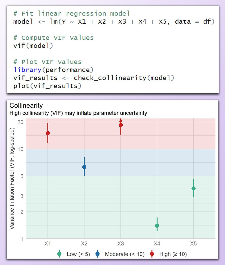The image below was created in R and shows a VIF plot categorizing predictor variables into low (green), moderate (blue), and high (red) multicollinearity. Variables X1 and X3 have high VIF values, indicating strong collinearity that should be addressed before interpreting the model. 🔹 In R, vif() from the car package computes VIF, while check_collinearity() from performance provides visualization. Ridge regression with glmnet can mitigate multicollinearity by applying regularization. 🔹 In Python, variance_inflation_factor() from statsmodels.stats.outliers_influence quantifies multicollinearity, and ridge regression with sklearn.linear_model.Ridge() helps stabilize estimates by penalizing large coefficients. Looking to improve your regression models? Check out my online course on Statistical Methods in R! Further details: statisticsglobe.com/online-course-… #R4DS #DataViz #Statistical #RStats #pythonlearning #Python #datavis #Rpackage

Urbanised landscape and microhabitat differences can influence flowering phenology and synchrony in an annual herb 🌿 Findings revealed that populations in urban sites exhibited earlier flowering onset compared to rural locations 🏢 👇 Read here: buff.ly/VWtG2kW

Validating habitat suitability models for pine marten (Martes martes) reintroductions to England and Wales 📈 The adaptive methodology can be applied to other species as reintroduction projects continue to grow in popularity 💭 🔗 doi.org/10.1111/1365-2…

New online! Drivers and solutions to Southeast Asia’s biodiversity crisis bit.ly/4o4alKA

Negative global-scale association between genetic diversity and speciation rates in mammals nature.com/articles/s4146…

In statistics, Frequentist and Bayesian approaches are two major methods of inference. While they aim to solve similar problems, they differ in their interpretation of probability and handling of uncertainty. Frequentist Approach: Frequentists interpret probability as the long-run frequency of events. Parameters (like the mean) are fixed but unknown, and inference relies on analyzing repeated samples. ✔️ Key Concept: Frequentist methods estimate a single, true parameter value based on hypothetical repeated sampling. ✔️ Confidence Intervals: A 95% confidence interval means that in repeated samples, 95% of intervals would contain the true value, not that there's a 95% chance for a single interval. ✔️ Hypothesis Testing: P-values measure how likely observed data (or more extreme data) would be under the null hypothesis. If the p-value is low (e.g., < 0.05), we reject the null. ❌ Limitations (Frequentist): P-values can be misinterpreted and do not directly indicate the truth of a hypothesis, and frequentist methods do not incorporate prior knowledge, limiting flexibility when such information is available. Bayesian Approach: Bayesians interpret probability as degrees of belief or certainty about an event, updated as new evidence emerges. ✔️ Key Concept: Bayesian methods start with a prior belief about a parameter, which is updated with data to produce the posterior distribution, reflecting the updated understanding. ✔️ Credible Intervals: A 95% credible interval means there's a 95% probability the parameter lies within this range, given the data and prior. ✔️ Incorporating Prior Knowledge: Bayesian methods incorporate prior information, making them flexible for combining expert opinions or past data. ❌ Limitations (Bayesian): The choice of prior can be subjective and influence results, and Bayesian methods often require intensive computation, especially for complex models like those using MCMC. The graph compares Frequentist Confidence Intervals (blue) from 20 samples with a single Bayesian Credible Interval (red). Frequentist intervals vary across samples, showing where the true parameter would fall in repeated sampling. In contrast, the Bayesian interval shows the 95% probability that the parameter lies within the range, given the data and prior. This highlights their different approaches to uncertainty. For more tips and insights on data science, sign up for my free newsletter! More details are available at this link: eepurl.com/gH6myT #datavis #DataViz #RStats #DataAnalytics

Our study ‘The #global #human impact on #biodiversity’ is out @Nature nature.com/articles/s4158… 🌍🌐🐟🌿🪲 🫎🦋🐝🪲 Unprecedented #synthesis of >2000 studies shows humans are not only shrinking species numbers—but reshaping entire communities across the planet. 🧵1/4

@RichHeydarian Voter turnout could also be a contributory factor. I wonder if there’s data on this.

(Fellow) MILLENNIALS —- and the Gen Z will DECIDE this ELECTIONS!!!

Take a moment to learn about the senatorial candidates before casting your vote. #Eleksyon2025 Get to know them here 👇philstar.com/headlines/2025…

Maximum Likelihood Estimation (MLE) is a fundamental method in statistics for estimating the parameters of a probability distribution based on observed data. The core idea is to determine the parameter values that make the observed data most probable under the assumed statistical model. How MLE Works: 1. Define the Likelihood Function: Given a statistical model with an unknown parameter (or parameters) θ and observed data X, the likelihood function L(θ; X) represents the probability of observing the data X given the parameter θ. For independent observations, this is typically the product of individual probabilities or probability densities. 2. Maximize the Likelihood: MLE seeks the parameter value θ̂ that maximizes the likelihood function. In practice, it’s often more convenient to maximize the natural logarithm of the likelihood function, known as the log-likelihood, due to its mathematical properties. 3. Solve for the Parameter Estimates: To find θ̂, take the derivative of the log-likelihood function with respect to θ, set it to zero, and solve for θ. This yields the parameter value that maximizes the likelihood of observing the given data. Example: Estimating the Mean of a Normal Distribution Suppose we have a sample of data points assumed to come from a normal distribution with unknown mean μ and known variance σ². The likelihood function for this sample is: L(μ; X) = ∏ (1 / √(2πσ²)) exp[-(xi - μ)² / (2σ²)] Taking the natural logarithm to obtain the log-likelihood: log L(μ; X) = -n/2 log(2πσ²) - (1 / (2σ²)) ∑ (xi - μ)² Differentiating with respect to μ and setting the derivative to zero: d(log L) / dμ = (1 / σ²) ∑ (xi - μ) = 0 Solving for μ gives: μ̂ = (1 / n) ∑ xi Thus, the MLE for the mean μ is the sample mean. Properties of MLE: • Consistency: As the sample size increases, the MLE converges to the true parameter value. • Asymptotic Normality: For large samples, the distribution of the MLE approaches a normal distribution centered at the true parameter value. • Efficiency: MLE achieves the lowest possible variance among unbiased estimators under certain regularity conditions. #Statistics #DataScience #Research #Science

In the 20 years since the term “microplastics” was first coined, a rapidly growing body of research has consistently shown how pervasive and problematic the pollutants have become. A new #ScienceReview provides an overview of this research and the progress made in understanding #microplastics. bit.ly/4doTICB

We've re-established our task group on on invasive alien species! @MelodieAM of @MonashUni will lead 11 experts in offering guidance & identifying pragmatic steps for GBIF to reach its full potential in supporting research & policy on #InvasiveSpecies: gbif.org/news/3AF5MJWHC…

Interested in how genomic data can help improve conservation assessments and population monitoring? Check out our paper in @EvolAppJournal where we outline background, provide a bioinformatic pipeline, and suggest an analytical framework🧵doi.org/10.1111/eva.70…

Basic statistics concepts (that all researchers should know)

#DYK that the USGS EROS Center has created an online #RemoteSensing classroom that provides students with a unique opportunity to explore the #Earth from a new perspective? Check out the #LandChange with #Landsat lesson here: ow.ly/nHoP50TeEAV #BackToSchool #OnlineLessons

Just a reminder that the 2009 Leaf Manual is available open access ! Use it and enjoy the leaves. 🍃🌿🍂 repository.si.edu/handle/10088/9…

Do you think that different types of data would produce different species’ range shift estimations? In this paper we can explore the differences in using abundance and occurrence data doi.org/10.1111/ddi.13… #ClimateChange #speciesdistribution #rangeshift #fishcommunities

We have a great list of ongoing award, fellowship and grant opportunities that we thought our members might be interested in. Check it out here: docs.google.com/document/d/1-x… #conservation #funding #fellowships #awards

A new #MachineLearning analysis has revealed the most effective climate policies out of 1500 implemented worldwide over the last two decades. Learn more in Science: scim.ag/89A

The training tool used in this study is an online app made with R Shiny, currently featuring nine plant diseases. It is freely available here: delponte.shinyapps.io/traineR2/