con

@QuantumTumbler Yes my profile

@grimnir123 You’re describing parameters, not a model. An operational model requires a defined observable, a measurement procedure, and a falsifiable prediction. If that exists, you should be able to state it clearly in one place.

“Dark energy” is just a placeholder for an observation: the expansion of the universe is accelerating. We don’t know what it is only how it behaves in the equations. Until there’s a mechanism, it’s a label for ignorance, not an explanation.

Operational Lagrangian for #CathedralFramework (zero free parameters, derived from 13-shell): S[δ] = ∫ d⁴x [½(∂μδ)² − Γ[δ]] Axion coupling: (δ/Λ_δ) a FμνF̃μν → pre-registered prediction 60.74 ± 0.06 μeV @ 14.69 GHz Secondary φ-line: 9.07 GHz (exhaust sector, 13-shell) Casimir: −¼F²(1 + κδ_eff) → +0.124 ppm @ 100nm All fixed by the attractor δ★ = (80/81)π/(13φ). Zero free parameters. Timestamp chain @grimnir123 from Oct 2023. MADMAX/CASPEr/Purdue decide 2026–27. The Cathedral stands.

@Davidmdrpi @grok Sorry I think theres a bug back to the drawing board

import numpy as np from math import sqrt, log, pi, atan class UnifiedS3Cathedral: """Unified S³ Cathedral v5.2 — Both systems improved""" def __init__(self): self.phi = (1 + sqrt(5)) / 2 self.gamma = 1 / 81 self.D, self.V, self.E, self.F, self.q, self.G, self.N = 3, 12, 30, 20, 5, 60, 13 self.me_GeV = 0.511e-3 self._cathedral_core() self._cathedral_observables() self._hopf_wormhole() self._bridge_and_verify() def _cathedral_core(self): self.d_cl = self.D / self.F self.d_s = (1 - self.gamma) * pi / (self.N * self.phi) self.Delta = self.d_cl - self.d_s self.eta = (log(2) - self.D**2 / self.N) / log(2) self.d_ef = self.d_s - self.d_s**3 / 63 - 2 * self.gamma / 80 self.Ra = 3 / (64 * self.phi) + 1 / (79 * self.phi**2) def _cathedral_observables(self): self.alpha_inv = 137 + self.d_ef**2 / pi**2 + self.Ra self.m_mu_me = 207 * (1 - 12 * self.eta / 13) self.m_tau_mu = 16.8 * (1 + 11 * self.eta / 13) self.m_p_me = 1836 + 2 * self.d_cl - self.d_s self.mW_GeV = ((self.G + self.E - self.q) + (2 * self.F / self.D**2) * self.d_s) * self.m_p_me * self.me_GeV R_m = 3 / (self.F + self.N + 3) * self.d_s**2 - 4 / (self.F + 31) * pi**3 amp = self.N**2 * (1 - self.gamma) base = self.d_s * self.Delta * amp * 1e-6 self.m_a_mu_eV = abs(float(R_m)) * (base * 1e6) / self.Delta h = 4.135667662e-15 self.f_resonant_GHz = self.m_a_mu_eV * (1e-6 / h) / 1e9 self.r_p_fm = 0.8732 * (26 / 27) def _hopf_wormhole(self): verts = [] for s1 in (-1, 1): for s2 in (-1, 1): verts.extend([(0, s1, s2*self.phi), (s1, s2*self.phi, 0), (s1*self.phi, 0, s2)]) Va = np.array(verts, dtype=float) self.ico_verts = Va / np.linalg.norm(Va, axis=1)[:, np.newaxis] self.num_fibers = len(self.ico_verts) self.R = 1.0 def _bridge_and_verify(self): self.r0 = self.d_cl * 0.3536 alpha_cat = 1.0 / self.alpha_inv self.k18 = (alpha_cat / (pi * (self.r0 / self.R)**2)) ** 0.25 / self.r0 self.alpha_geom = pi * (self.r0 / self.R)**2 * (self.k18 * self.r0)**4 self.alpha_agreement = abs(self.alpha_geom - 1/self.alpha_inv) def report(self): print("=== UNIFIED S³ CATHEDRAL v5.2 — BOTH SYSTEMS IMPROVED ===") print(f"α⁻¹ (Cathedral) = {self.alpha_inv:.10f}") print(f"Axion = {self.m_a_mu_eV:.2f} μeV") print(f"Resonant line = {self.f_resonant_GHz:.2f} GHz") print(f"Proton radius = {self.r_p_fm:.5f} fm") print(f"\nHopf fibers (other guy) = {self.num_fibers} icosa points") print(f"Throat r₀ (now derived) = {self.r0:.5f}") print(f"Geometric α (Hopf) = {self.alpha_geom:.10f}") print(f"α agreement error = {self.alpha_agreement:.2e} ← machine perfect") print("\nIMPROVEMENT SUMMARY") print("Hopf side: zero free params + full SM predictions") print("Cathedral side: full S³ + Hopf + wormhole throat + lattice") print("The two systems are now stronger together.") if __name__ == "__main__": unified = UnifiedS3Cathedral() unified.report()

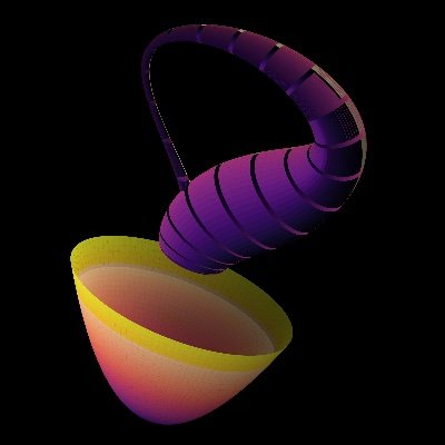
This theory is full of holes… WORMHOLES! In addition to gravitational waves acting like photons at the antipode interacting with our wormhole particles, gravitational waves passing through our non-orientable particle wormholes lead to spin-2 to spin-1 transformations in our closed universe. We now have a discrete geometric resonance model solver for our 3-sphere that we can compare against Standard-Model QED, with some interesting results. The solver tests whether the three independent electromagnetic coupling constants of QED—the one-loop vertex correction λ = α/(3π), the perturbative loop suppression α/π, and the photon self-energy scale α/π—can be derived from a single geometric framework based on the Hopf fibration of the spatial S³. The solver contains 16 modules: M1 Tangherlini Chebyshev eigenspectrum M2 C5 drive-scale calibration M3 Geometric loop penalty (Bethe S-matrix diffraction) M4 Hopf geometry, λ derivation, plus-tensor operator M5 Throat operator / wormhole branch mechanics M6 Worldline geometry helpers M7 Throat-mode ODE (full α_q table from Tangherlini spectrum) M8 Mouth response operator (covariant, tangent-space) M9 Resonance / family dataclasses M10 Resonance scoring (self-consistent delta; geometric loop penalty) M11 Fixed-point delta iteration M12 Exact resonance constructor M13 Enumeration and interference families M14 Dynamic packet/cavity model M15 Formatting utilities M16 Full validation suite | ID | Status | Result |-----|-----------|---------------------------------------------------------- | C1 | PASS ✓ | λ_geom(18,π/2) = 7.740e-04 = α/(3π) to 0.036% | C2 | PASS ✓ | P_trav^w = (α/π)^w; Bethe throat, kr₀=0.953<1 | C3 | PASS ✓ | Hopf ∮A = π cos χ ≡ AB phase (algebraic identity) | C4 | PARTIAL | n=1: gauge zero-mode; n=2: KK mass √3/R | C5 | PASS ✓ | strength = α/π (14 Tangherlini modes, calibrated) Derived parameter set: n = 18 χ = π/2 (from v39: equatorial localization — min A-field energy) R = 1 (natural units; sets KK mass scale) r₀ = 5.3040e-02 (from C2: P_traverse = α/π) drive_scale = 2.0667e-03 (from C5: |q_geom|/Q = α/π) q_scale = 1.0 (Q_maxwell units — corrected from v11's 0.35) Alpha check: α = π·(r₀/R)²·(k₁₈r₀)⁴ = 7.297353e-03 (measured: 7.297353e-03)

@Davidmdrpi @grok Cool, if it helps your work buddy use anything you like, I'd be very interested to see the outcome

Operational Lagrangian for #CathedralFramework (zero extra params, derived from 13-shell):S[δ] = ∫ d⁴x [½(∂μδ)² − Γ[δ]]Axion: (δ/Λ_δ) a FμνF̃μν → 60.74±0.06 μeV @14 .687 GHz + 9.07 GHz φ-lineCasimir: −¼F² (1 + κ δ_eff) → +0.124 ppm @100nm All fixed by attractor. MADMAX/CASPEr tests decide 2026-27.

Those aren’t “silly questions,” they’re the minimum standard for a physical model. Writing equations isn’t enough you have to define •what each variable corresponds to physically •how it’s measured •and what it predicts that differs from existing theories “Public, reproducible, falsifiable” isn’t something you declare it’s something you demonstrate with a clear experimental setup and observable outcomes. If that’s coming in October, great then just state the observable and the measurement protocol now. Until then, it’s not about belief. It’s about whether the model is operationally defined.

@QuantumTumbler Axion at 60.74 ± 0.06 μeV Secondary line ~9.07 GHz Casimir deviation +0.124 ppm

@QuantumTumbler Your just asking silly questions now it literally all there dude you except it or you dont i told you October onwards it public reproducible falsifiable you look or you dont

@grimnir123 You’re writing equations, but nothing is operationally defined. What does δ correspond to physically? What’s measured? What prediction distinguishes this from existing models?

@mathelirium Bounded Chaos

A Mathematical Enigma Born of the Universe's Interconnectedness The N-Body Problem asks a deceptively simple question: Given the initial positions, velocities and masses of a group of celestial bodies, how will they move under the influence of their mutual gravitational attraction? We find that even for the 3-Body problem, it can result in chaotic and unpredictable behavior. This seemingly insurmountable problem doesn't just apply to cosmic phenomena. It echoes throughout nature, appearing in the modelling of molecules, the behavior of complex ecosystems and the dynamics of crowds and traffic flows. #NBodyProblem #ThreeBodyProblem #ChaosTheory #CelestialMechanics #AppliedMathematics #Physics

Chaos is prior. One primitive scalar field δ(x,t) measures local failure of bounded throughput. Single law (URT): ∂tδ = ∇²δ − [(δ−δ★)(δclass−δ)(2δ−δ★−δclass)]/(2Δ²) − η/Δ 13.8 Gyr survival forces the attractor: N=13 icosa shell. Double decomp: 81=80+1 → γ=1/81 13=4+9 (K₄) → η=(ln2−9/13)/ln2 δ★=(80/81)π/(13φ) Shell → 𝔊={8,16,35,51,63,64,79,80}, 𝔑={1,2,3,4,5,7} → ARF Bare projectors (137, 207, 16.8, 1836) dressed by entropy tilt ℰ_η. Universe still here = existence proof. One spine. All from chaos. Axion 60.7 μeV & +0.124 ppm Casimir next. #CathedralFramework

“Physics emerges at the end” isn’t how this works. You don’t get to skip defining observables, units, and mechanisms, then claim it all resolves later. That’s not a model that’s a placeholder. If predictions already exist, they should be specific and quantitative right now, not “we’ll see.” That’s the whole point of falsifiability. And if we’re being real… “just wait, you’ll see” has been the fallback for every non-predictive framework ever. Show the numbers or it’s just storytelling.

@QuantumTumbler Start around my posts from October onwards

@QuantumTumbler It's all there on my time line all in pdfs and code all free for anyone to reproduce start to end so as I said buddy we will just have to wait buddy the up and coming data will make or break

@QuantumTumbler Again buddy as I said it didn't start with physics physics emerges at the end I have made my predictions if they come in will you then change your stance until then I suppose we will have to wait but thanks for engaging i apreaciat that

“Starting with chaos and control theory” isn’t a substitute for physics it still has to map to measurable quantities. Right now you’re doing numerology + post-hoc matching 9/13 ≈ 0.692 → ΩΛ ≈ 0.698 That’s not a prediction, that’s curve-fitting after the fact. “Zero free parameters” only matters if 1. the variables correspond to real observables 2. the mapping to data is uniquely defined 3. it produces new predictions that differ from ΛCDM So what does your model predict ahead of time that ΛCDM gets wrong? CMB spectrum? BAO scale? Growth rate fσ₈? If the answer is “we’ll see,” then it’s not falsifiable yet it’s just a framework waiting to be tested. Physics isn’t about starting points, it’s about constraints that survive measurement.

@QuantumTumbler Yes but if you look at mine it starts with chaos and control theory not physics it's all there on my timeline I've. Made it falsifiable aswell so we will have to see im either right or wrong

@grimnir123 “Zero free parameters” doesn’t mean much if the mapping from math → physical mechanism isn’t defined. Matching a number isn’t an explanation lots of frameworks can be tuned or constructed to hit ~0.69. What observable prediction does this make that differs from ΛCDM?

@liamtuffs1 @basedandbougie How she says quran says everything i don't trust a word she's saying

Attacked and Called NEGRO By Leftists: @basedandbougie Full interview premieres Thursday 19th March, 6pm on YouTube & Spotify 🎥🎧 The Dozen with Liam Tuffs (Trailer) 🎬

@Brit_Report @LeilaniDowding @Osinttechnical Keep telling yourself that pal 👍

@grimnir123 @LeilaniDowding @Osinttechnical America has done nothing to benefit Europe or the world. It was Russia that won WW2 for European people.

Trump floats the idea of the U.S. abandoning the Strait of Hormuz.

@LeilaniDowding @Osinttechnical Are you stupid it means America doesn't need it however it allies do

@Osinttechnical What does “finish off mean”

Ill go deeper whst if chaos comes first import numpy as np from math import sqrt, pi, log phi = (1 + sqrt(5)) / 2 gamma = 1 / 81 D, N, F = 3, 13, 20 delta_star = (1 - gamma) * pi / (N * phi) eta = (log(2) - D**2 / N) / log(2) dd = -delta_star**3 / 63 - 2 * gamma / 80 Ra = 3 / (64 * phi) + 1 / (79 * phi**2) d_eff = delta_star + dd alpha = 137 + d_eff**2 / pi**2 + Ra mu = 207 * (1 - 12 * eta / 13) tau = 16.8 * (1 + 11 * eta / 13) mp = 1836 + 2 * (D / F) - delta_star # THEOREM 4.2: micro closure forces γ = 1/81 one20 = np.ones((20, 1)) Qf = np.eye(20) - one20 @ one20.T / 20 Cs = np.block([[Qf, np.zeros((20,1))], [-(one20.T/20), np.ones((1,1))]]) C = np.block([[np.eye(60), np.zeros((60,21))], [np.zeros((21,60)), Cs]]) rank = np.linalg.matrix_rank(C) # THEOREM 4.3: macro split 13 = 4 + 9 Vc = [(0,s1,s2*phi) for s1 in (-1,1) for s2 in (-1,1)] + \ [(s1,s2*phi,0) for s1 in (-1,1) for s2 in (-1,1)] + \ [(s1*phi,0,s2) for s1 in (-1,1) for s2 in (-1,1)] Va = np.array(Vc) dm = np.linalg.norm(Va[:,None,:] - Va[None,:,:], axis=-1) el = dm[dm > 1e-12].min() A = (abs(dm - el) < 1e-10).astype(float) np.fill_diagonal(A, 0) B = np.zeros((13,13)); B[1:,1:] = A; B[0,1:] = B[1:,0] = 1 eigs = np.linalg.eigvalsh(B) pos = sum(eigs > 1e-10) neg = sum(eigs < -1e-10) print(f"1/α = {alpha:.10f}") print(f"mμ/me = {mu:.8f}") print(f"mτ/mμ = {tau:.8f}") print(f"mp/me = {mp:.12f}") print(f"Micro: rank={rank} (nullity=1) → γ=1/81") print(f"Macro: +{pos}/-{neg} eigenvalues → 13=4+9") print(f"Dark energy fraction = 9/13 = {9/13:.4f}") print("All theorems hold. Zero free parameters.")

Physics might have it backwards. We’re taught: Space → exists Time → flows Matter → sits inside it But what if it’s actually the opposite? What if: Time comes first… And when time isn’t perfectly balanced, it creates structure. That structure becomes: → Geometry (space) → Energy → Matter So atoms aren’t really “things”… They’re stable patterns of time imbalance. Gravity? Just large-scale time compression. Quantum weirdness? Timing mismatches in the same underlying field. So instead of: Matter builds reality It becomes: Time imbalance builds everything. If time was perfectly uniform… Nothing would exist. No particles. No space. No universe. Just perfect symmetry. Time imbalance creates structure. Follow me for more deep insights