LA Genchev

@Andromeda_Macro Have you guys changed your views after Trump's speech this evening?

We're looking for: * S&P 500 - 6,200 (-6% from current) * Brent - $150 (on spike) * US 10yr 4.5% * EUR-USD 1.12

Morning Call: * Brent touches $118 as conflict continues * SPX futures down 1.3% * Gold lower -1.4% from margin driven selling * Bond yields sharply higher (US 10yr +5bps, UK +13bps) * DXY stronger as safe haven demand continues Not max pain yet.

@NoAlphaLimits Thanks for the insights. What is the data source for your drone/missile numbers?

@junkbondinvest Total horsesh!t...

Denmark gov't bonds at 48 cents. When a country's debt trades below 50, you start eyeing the collateral. Greenland is the collateral.

Why is everyone talking about the treasury basis trade. The treasury basis trade is, to a first approximation, fine. The thing that is blowing out is swap spreads.

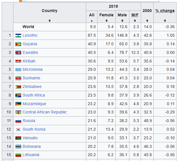
@ulriklykke Can you please share some source for the highest suicide rate and alcohol consumption per capita? I see different numbers online. For example here's the ranking for "Highest suicide rates per capita": (not claiming wikipedia is perfect)

Credit first and foremost is about availability, and only then does price come into play. THE SINGLE MOST IMPORTANT FACTOR right now is the abundance of availability. It will also be the topping signal. The price rug pull will only come after the availability rug pull. 1/3

@Daniellaaadolly @kos_data This is the dumbest thing ever..

@kos_data Romania and Serbia do not exist. Fixed Balkan Paris Olympic Medals: 🇧🇬 15 🥇🥇🥇🥈🥉🥉🥉🥇🥇🥇🥈🥉(+5) 🇧🇬 7 🥇🥇🥇🥈🥉🥉🥉 (+1) 🇭🇷 6 🥇🥇🥈🥉🥉🥉 🇬🇷 8 🥇🥈🥉🥉🥉🥉🥉🥉 (+1) 🇸🇮 2 🥇🥈 (+1) 🇹🇷 7 🥈🥈🥈🥉🥉🥉🥉 (+2) 🇲🇩 4 🥈🥉🥉🥉 🇽🇰 6 🥈 🥇🥇🥈🥉( +2) 🇦🇱 1 🥉 (+1) 🇧🇦 0 🇲🇪 0 🇲🇰 0

Balkan Paris Olympic Medals: 🇷🇴 8 🥇🥇🥇🥈🥈🥈🥈🥉 🇧🇬 7 🥇🥇🥇🥈🥉🥉🥉 (+1) 🇭🇷 6 🥇🥇🥈🥉🥉🥉 🇷🇸 4 🥇🥇🥈🥉 (+2) 🇬🇷 8 🥇🥈🥉🥉🥉🥉🥉🥉 (+1) 🇸🇮 2 🥇🥈 (+1) 🇹🇷 7 🥈🥈🥈🥉🥉🥉🥉 (+2) 🇲🇩 4 🥈🥉🥉🥉 🇽🇰 2 🥈🥉 🇦🇱 1 🥉 (+1) 🇧🇦 0 🇲🇪 0 🇲🇰 0 (10 August)

@torikeqi @pabloonorris @kos_data You really are a clueless racist 🤦🏼‍♂️

Balkan Olympic Medals 2024: 🇷🇴 8 🥇🥇🥇🥈🥈🥈🥈🥉 🇧🇬 6 🥇🥇🥈🥉🥉🥉 (+6) 🇭🇷 6 🥇🥇🥈🥉🥉🥉 🇷🇸 2 🥇🥇 🇬🇷 7 🥇🥈🥉🥉🥉🥉🥉 🇸🇮 2 🥇🥈 (+1) 🇹🇷 5 🥈🥈🥉🥉🥉 (+1) 🇽🇰 2 🥈🥉 🇲🇩 3 🥉🥉🥉 (+1) 🇦🇱 0 🇧🇦 0 🇲🇪 0 🇲🇰 0 (9 August)

🇧🇬🥇 Bulgaria has another Olympic champion!!! 💪 Carlos Nasar is No 1 in weightlifting setting world records along the way

@richfalkwallace Hi Rich! Would appreciate the excel!

"Orthogonalization" The problem statement is: You have a risk model that divides both forward risk and historical performance into systematic and idiosyncratic components. And you have decided to manage those core model factors in whatever way you want, anywhere along a spectrum from simple awareness to intraday neutralization. But you would now like to drill deeper into the idiosyncratic component of risk & performance: 1) Are there any systematic exposures buried inside idio not already captured by the factors you are using in your core risk model? 2) Can you explain some of the realized historical idiosyncratic performance as a function of aspects that are not purely company-specific? The first question runs into an ongoing debate about 'parsimony' in risk models: what set of risk factors explains systematic risk without overloading a factor model with so many (and so rapidly changing a set of) factors that it is impossible to actually manage a portfolio against? The second runs up against the deeper question of what it means for a return to be factor-driven vs. idiosyncratic. Ultimately, how to truly divide alpha and beta. The details of those debates can be settled another time. But in the context of those questions, “orthogonalization" (or "residualization") exists to allow yet another layer of decomposition more granular than factor vs idio, this time to decompose the idiosyncratic component itself. Why would you want to do this? A few reasons: For discretionary investors, the reality is you are intimately aware of many more systematic drivers of your stocks than can be captured in core style & industry factors. Orthogonalization captures exposures & performance associated with industry-specific datasets or macros you care about, nuances around consensus estimate revisions, varying momentum windows, options signals, and of course, crowding - either globally or sector-relative. In principle, each of those items could of course be integrated into a core risk factor set, explicitly limiting exposures & pro forma vol against each of those more nuanced, custom factors. But in practice, most firms that care intensely about these topics perform this separation of factor-types using orthogonalization: A relatively parsimonious set of core style & industry risk factors against which books must be managed. And a more extensive set of custom orthogonal factors that are used as awareness and insight tools, but do not limit risk taking. All of which produces a proactive as opposed to reactive approach to factor risk & performance, and to understanding the drivers before they become the only thing you can focus on. The sheet walks through orthogonalization math, building from the earlier factor model to layer in custom loadings, returns, and attribution. With strong engineering & data infrastructure, the math is doable. What you do with it is a different question. Let know if you'd like the excel.

@richfalkwallace @__paleologo thank you for the post! would appreciate the excel too

Risk models increasingly drive the behavior of fundamental long short equity investors. @__paleologo's 'Advanced Portfolio Management' is the most efficient primer to understand the internals of what is happening. Chapter 1-4 bullets, with math & comments. Let know if you'd like the excel. *1) Risk, alpha, factors, & performance (Ch 1-3)* "Any argument in favor of conflating beta and alpha is weaker than the simple argument in favor of decomposing them." In the simple version, stocks contain components of both: 1) Systematic (factor) returns driven by common attributes across names, and 2) Idiosyncratic (residual) returns driven by specific attributes of each. Most investors accept this distinction at a high level. But the nuance is: How sophisticated should your modeling of this "systematic" component be? The first intellectual step beyond simple benchmarking is to look at historical beta: running a univariate regression between stock & market. But simple betas are imprecise for several reasons, among them that they conflate one-time idio moves with recurring systematic relationships; and they also gloss over other often large systematic drivers (industry, growth, value, momentum). Factor models in principle address those limitations: If a simple benchmark "gives us a way to describe performance and variation of stock returns," the solution is "factor models[, which] capture these two intuitive facts, make it rigorous, and extend them in many directions." *2) How to build a factor model (Ch 4)* There are many flavors of plausible factor models, and Gappy outlines 3 (fundamental/characteristic, statistical, time-series). As Gappy points out: "Each of these approaches has its merits and drawbacks" and he covers several of the core tradeoffs at the outset of the chapter. 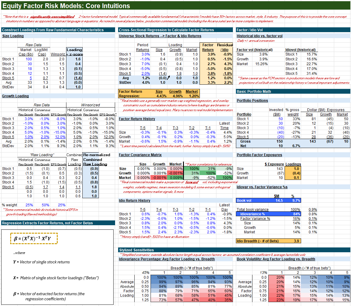But "the characteristic model has the benefit of being interpretable by the managers" and "can be extended with new characteristics and perform quite well in practical applications." The result is that "because of these two decisive advantages, the fundamental (or characteristic) method is by far the most used model by fundamental managers." To build a fundamental factor model, the starting point are company attributes which are transformed into "loadings" (betas) of a stock to that attribute's returns. For example: The "size" loading is the simplest factor, and starts with the log of the stock's market cap compared to other market caps in the universe you care about. The size loading is then its z-score (# of standard deviations away from avg) in that universe. (In the weeds, data is winzorized, may use EWMAs, and more). But armed with those loadings, the model then pulls factor returns by running cross-sectional regressions of stock returns against their loadings. Restated in math: The Y vector is each stock in the universe's return over the period, The X matrix is all of their loadings. The time series of those extracted factor returns then drives factor covariances (the FCM), residual returns, mimicking portfolios, idiovar%s, breadth, vol, and more. There is much more worth spending time on here, but particularly to arm the fundamental investor with the basic mathematical intuitions, I've attached a very simplified fundamental factor model. Will cover many other topics Gappy touches on another time: attribution, sizing skill, factor detail, PCAs & non-linearity, Sharpes & ICs, optimization, vol, & leverage. But stepping back, the reason this all matters is simple: "empirically, most PMs have no skill in style factors whatsoever, and a few have very moderate skills in having exposures to industries or sectors." The book's meta theme is intellectual honesty: "The simplest and deepest challenge is to understand the limits of your knowledge." Factor models rigorously separate what analysts can predict about single stocks, from what they cannot. As Gappy points out, "you are entering an industry in transition." Let know if you'd like the excel.

@nope_its_lily @quantymacro @macrocephalopod Do you find just the tests useless or the concept of cointegration as a whole? I.e. do you find error-correction models useful in practice? (i have)

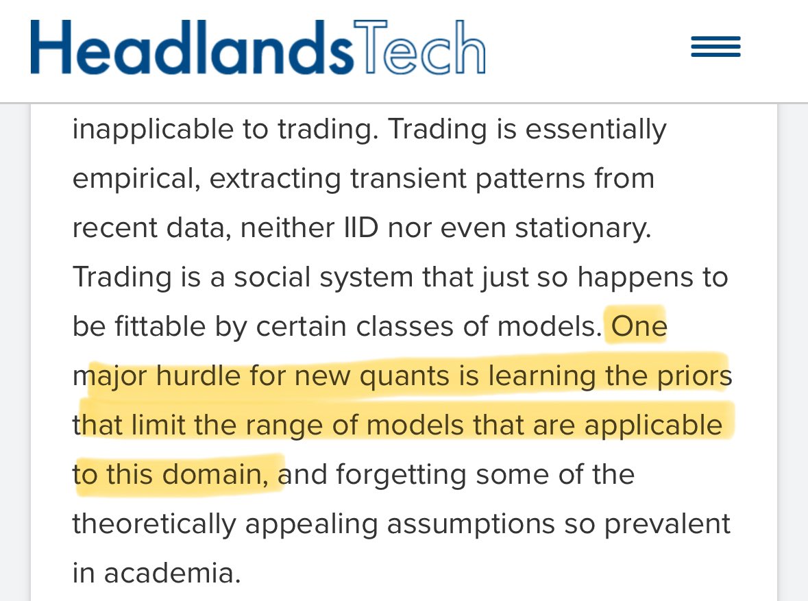
ok timeline cleanse from white noise mean reversion. was reading Max Dama’s ESL review, & thought this part was good my takeaway is you need two things: 1) models that work in finance 2) models that *you* can make it work stop saying XTX or RenTech to justify *you* doing RNN

@elonmusk When is the interview coming out??

So hot rn

Calling it now, there is a close to 100% chance that this fund is a scam.

@richfalkwallace Yes pls

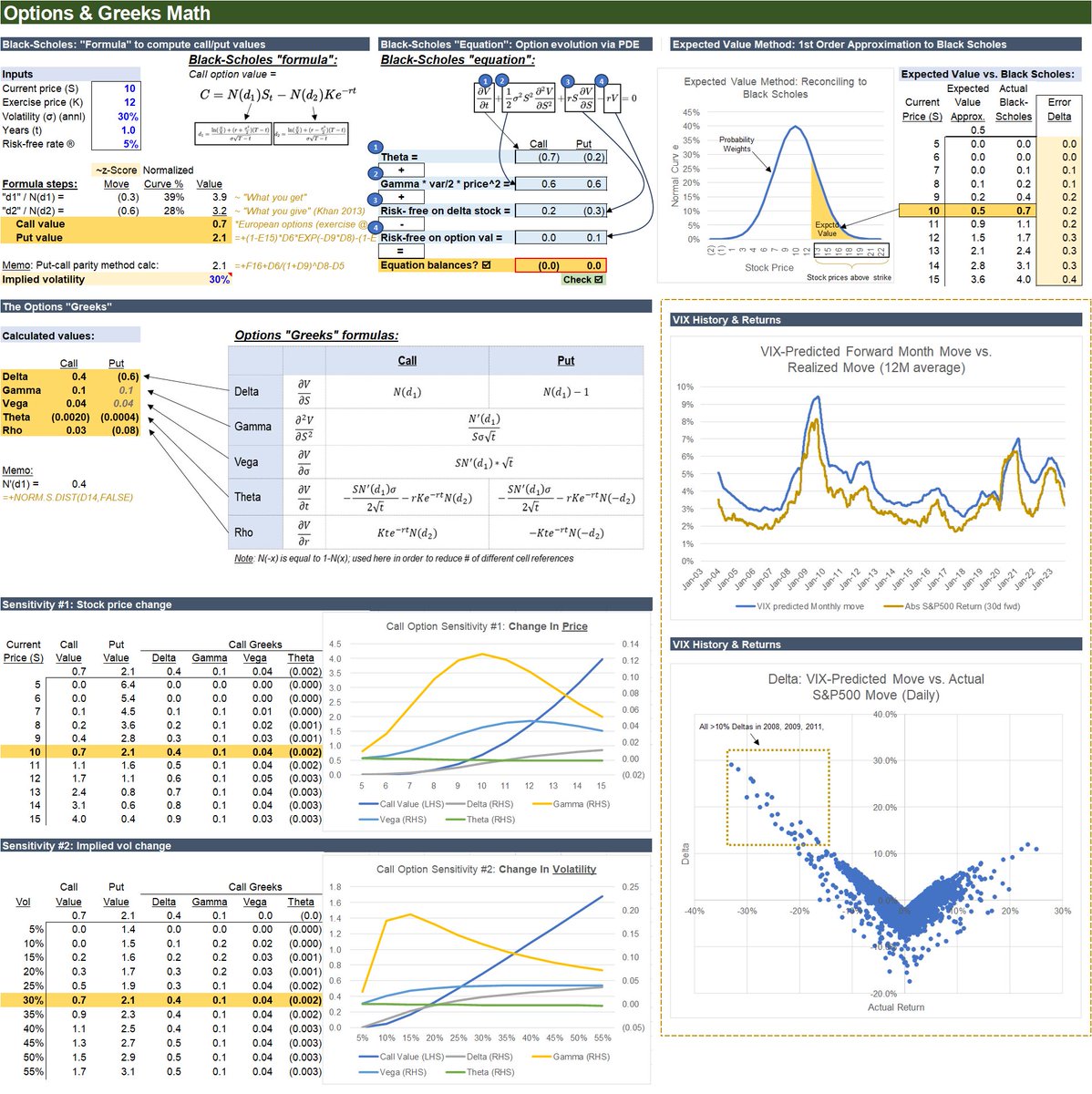
If you don't understand options & greeks, you don't understand markets Comment if you'd like the excel *Updated* 6 points: The update: The VIX today sits at 12.6, 35% below its 20yr avg and at its 16th percentile historically. Which implies a ~3% expected value 1 month S&P move. How accurate is that VIX prediction typically? And when does it fail? 6 points: 1) First Principles An option is the right to buy or sell a stock at a pre-specified price. So if a stock is trading at $10, a call option with a strike of $12 and 1 year to expiration - Is clearly worth something. But how much? 2) Black-Scholes 'Equation' The primary answer is Black-Scholes. In math, it describes two competing forces in an option's value: The negative force is decay of the option's value over time (its "Theta") The positive force is growth in option value as the stock moves (#2 multiplying Gamma by vol & price - a price-nonlinearity analogous to bond "convexity"). Leaving aside risk free return, the core insight is this: The negative change from time decay must exactly offset the positive change from Gamma's nonlinearity. You can watch that tradeoff (partial differential equation) balance exactly in cell N20. 3) Black-Scholes 'Formula' The most practical form is the solution to this PDE calculating the value of call/put options. Simplifying to a first order approximation, that formula asks: What is the probability that this option ends up profitable - And then multiplies that by the difference between the expected value of the stock in that scenario and the exercise price. This math reconciles exact Black-Scholes to the expected value approximation in cell X6. 4) Greeks Greeks show how options move with their inputs: Delta = option move per change in the stock Gamma = how delta itself moves with the stock Vega = option move per 1% change in vol Theta = option move per day that passes Other less common Greeks capture their rates of change (higher derivatives). 5) VIX The VIX approximates front month implied volatility of the S&P500. Bottom right charts its history. The first is the VIX-predicted S&P move, Against the realized absolute move. Averaged & smoothed, they move in lock step, with a delta equal to the ‘volatility risk premium’. The daily data is messier: Implied vol has an ~18% R^2 to realized vol - high but far from perfect. The 2nd chart shows predicted minus absolute move, Compared against realized returns. The key point: The largest misses happen in the worst markets. 6) Beyond Investors use options to express directional views, hedge, or take explicit vol positions (surface trades, carry/dispersion). And also serve as metaphors for a wide range of payouts. There are limitations and depth in every direction here. As always, the key is a firm grasp of principles, Clarity on the math, And intellectual honesty about the limitations. That's all for now Comment if you'd like the excel

@PatrickJamesGNG @TaylorLewan77 @Coach_SMoore You have to give the guy some breathing room... Also don't post photos of your fat belly and you won't get flagged.

@TaylorLewan77 @Coach_SMoore He’s right on that line of acceptable male crying. Almost an ugly cry, which would be a flag every time.

Incredible to see the love and emotion this man has for the players/university. @Coach_SMoore is gonna be an incredible head coach in the future, but for now I’m so damn glad he’s a Michigan Wolverine.

Select numbers between 0 and 1 randomly until sum is > 1. The expected # of selections needed is equal to e.

@richfalkwallace Send it over please 🐥

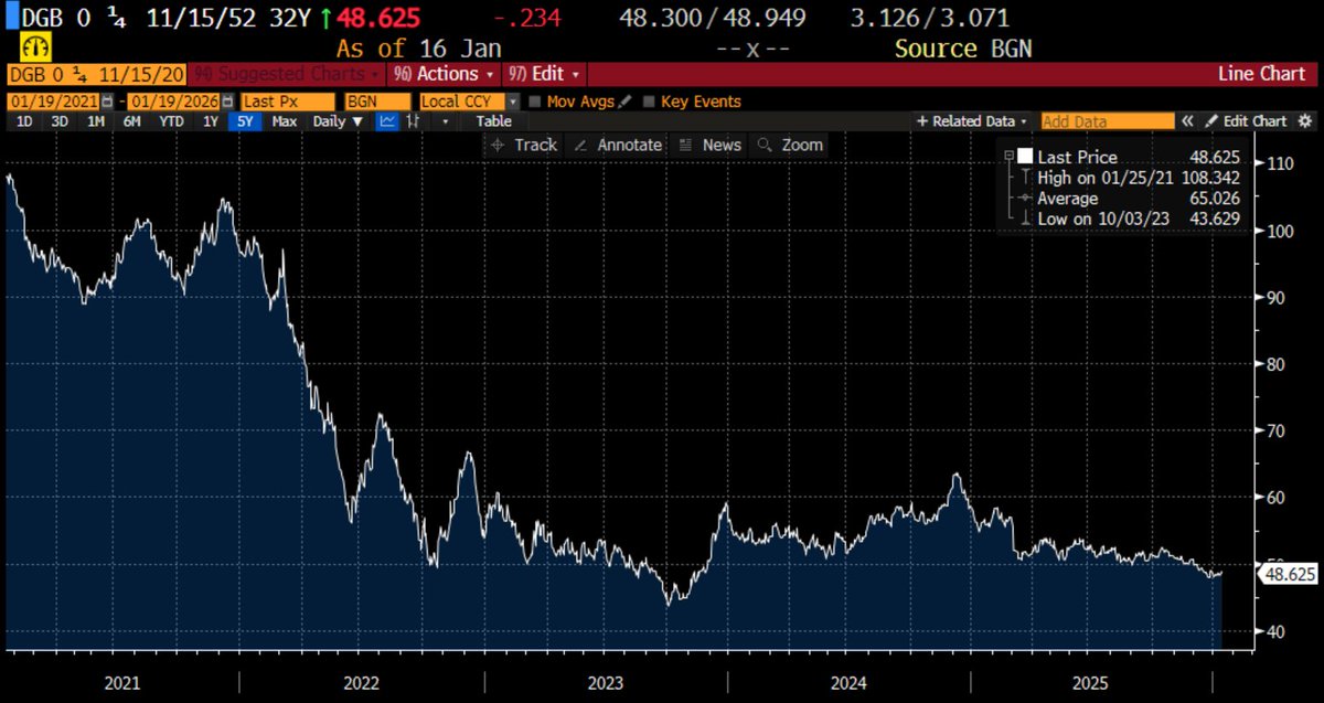
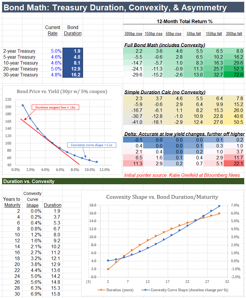
Bond math is now key to today's financial markets Let know if you'd like the sheet. The table on the right reflects a powerful new dynamic: If rates fall 50bps, 20yr Treasuries earn 11.3% over the next year. But if rates rise by 50bps, they lose just 0.9% -- an 11:1 up/down ratio. The 5 year-average 20yr yield is just 2.5%, compared to today's 5%+ yield. At that lower history, the same 50bps up/down math sat at just 2:1, much less skewed. So in the context of recession fears, commodity shock, and mixed econ data, that return skew is drawing cross-asset investors -- hedge funds & asset managers normally less involved in Treasuries. This competition for capital is one of many mechanisms by which higher rates challenge equity returns. Several items are pushing long rates up: the rise of JGB long rates, US deficits, persistent inflation, the dollar, and others. But implicit in the new investor framing of long-bond risk/reward is also the changing impact of the duration math, and the role of convexity across the curve. Which is worth understanding. Duration describes the average time it takes to receive any set of cash flows. Whereas a bond's maturity is simply the date principal is repaid. As a result, maturity and duration differ if there is a coupon: the larger the coupon relative to the principal (& price), the shorter the relative duration. So, if a 10yr bond at par has no coupon, its duration is 10 years. If the same bond has a 10% coupon, its duration is 6.5 years, since much of the total cash investors get comes in every year via coupon. But the duration has another very useful property: It also exactly equals the bond price change associated with a 1% change in its yield. Thus, for the same 6.5 year duration bond, if the yield falls to 9%, the price rises from 100 to exactly 106.5. The next question is how duration changes: Is the 6.5 duration constant as yields move from 10% to 9% to 8%? No -- because the weighted average life has changed at each increment. This change is the bond's "convexity." And it is the driver of why a 3% rate fall means a gain of 70%+ while a 3% rise means a loss of just 30%. You can see that difference in the first chart below: Red is the duration of a 5% coupon / 5% yield 30-year bond: 16 years. Blue is the actual bond price across yields. The difference between the two lines is the effect of convexity: The price change slows as yields rise And rises steeply as yields fall. Next shows the curve of convexity itself shifting across maturities. Directional views on Treasuries here are a function of growth path, fed policy, and a host of other factors. Sometimes you make that bet. But other times, or if you're restricted to markets competing for scarce capital, Knowing the asymmetries & reaction functions across markets Improves your ability to anticipate and act In your area of focus. That's all for now. Let know if you'd like the math.