0xSplayTreee

I'm: - Web Developer 🌐 - Software Developer 👨‍💻 - AI & Machine Learning Engineering Student 🧠 - Cybersecurity Analyst Pro 🕵‍♂️ - BSc in Computer Science 🧮 - Starting a Graphic Design Degree 🎨 - Future Mathematician (Cryptography Theory) 🧮 🧠 🕵‍♂️

The Fundamental Theorem of Calculus connects the two core ideas of calculus: derivatives and integrals. If A(x) = ∫ₐˣ f(t)dt then d/dx[∫ₐˣ f(t)dt] = f(x) As x moves, the integral gains a tiny strip of area. That strip is approximately f(x)·dx, so the rate at which the total area grows is simply the height of the curve at x. One elegant theorem unites accumulation and change, forming the foundation of modern calculus.

Spring setups control how a system resists force and how quickly it bounces back. In series the effective spring constant follows the relation 1/k = 1/k₁ + 1/k₂. In parallel the effective value is the sum k = k₁ + k₂. The angular frequency of oscillation for an attached mass m is given by ω = √(k/m) using the effective k. It is used to determine the natural frequency of vibration in mechanical devices such as engine mounts and building dampers.

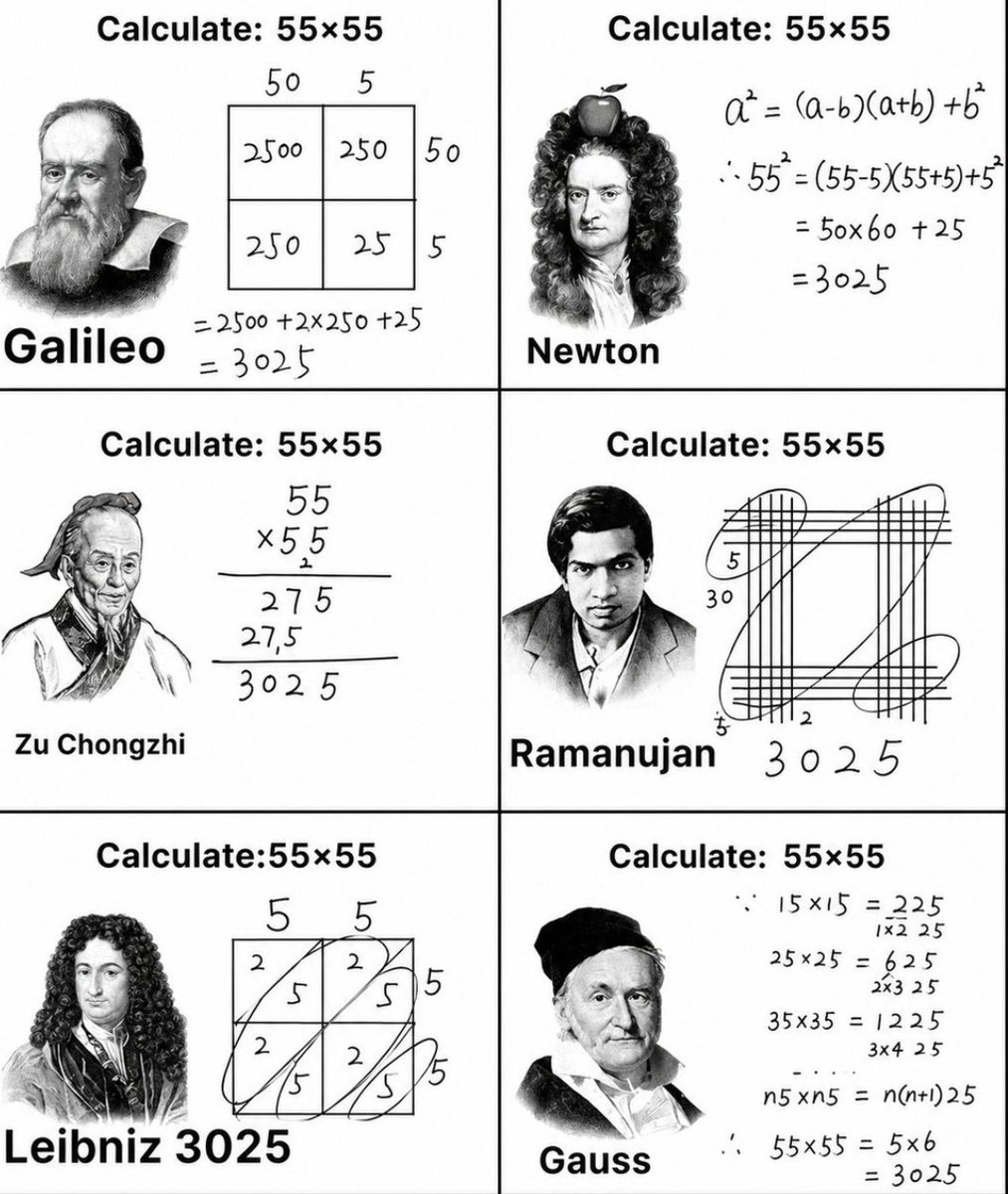
Imagine asking some of history's greatest mathematicians just one question: What is 55 × 55? Galileo Galilei, Isaac Newton, Zu Chongzhi, Srinivasa Ramanujan, Gottfried Wilhelm Leibniz, and Carl Friedrich Gauss might each solve it in their own unique way, yet every path leads to the same answer: 3025. Different minds. Different methods. One correct result. Which approach would you choose?

Timing is everything.

Your parents will be alive to see you win big, Amen.

Monthly investing vs. Waiting for 20 & 40% crashes since 1993

Sunday wisdom lol

Be like the Ant, proverbs 6:6-11

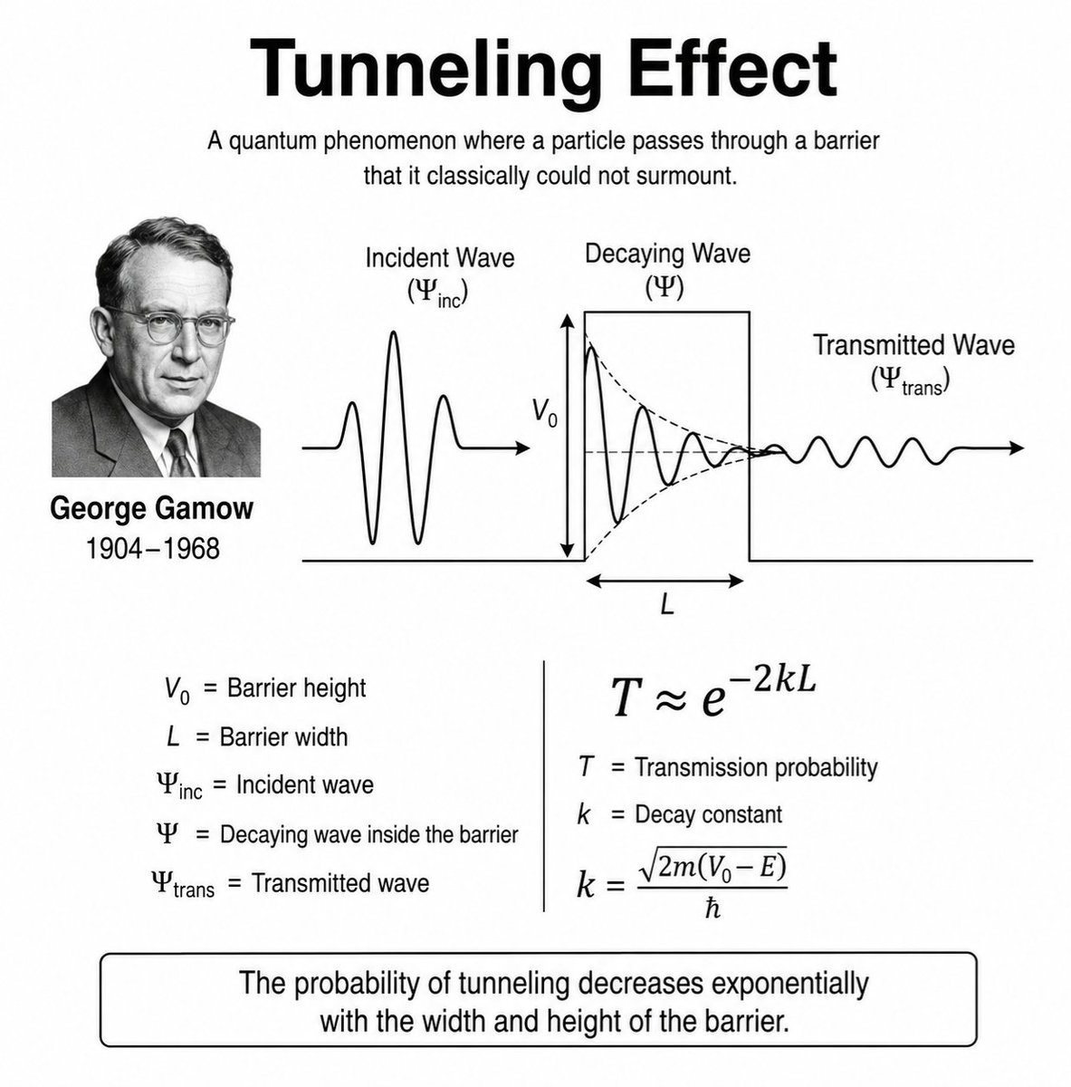
Quantum tunneling is the phenomenon where a particle has a finite probability of passing through a potential barrier, even when it doesn't have enough energy to overcome it classically. The tunneling probability is approximately : T ≈ e⁻²ᵏᴸ where, k = √(2m(V₀ − E)) ⁄ ħ Here, T is the tunneling probability, L is the barrier width, V₀ is the barrier height, E is the particle's energy, m is its mass, and ħ is the reduced Planck constant. The equation shows that tunneling becomes exponentially less likely as the barrier gets wider or higher. This quantum effect explains alpha decay and makes technologies like tunnel diodes and scanning tunneling microscopes possible.

Post your ZLib recommendations!

By age 27, you should be smart enough to realise this:

Dual nature of matter explains that light shows particle properties, while matter also exhibits wave-like behavior. These equations summarize the key concepts of photon energy, the photoelectric effect, photon momentum, emitted photon energy, and hydrogen atom energy levels.

17 Equations That Changed The World. By Ian Stewart.

If you're a backend engineer, Please learn: > SOLID design principles > Multithreading > Immutability > Streaming & messaging > Caching > Idempotency > Security > SSL, JWT, OAuth > Design patterns (Factory, Decorator, Singleton, Observer/Observable) > TDD (Test-Driven Development)

A tensor is a mathematical object that represents physical quantities in a way that remains unchanged under a change of coordinates. It generalizes scalars, vectors, and matrices into a single mathematical framework. You can think of tensors by their rank. Rank 0: Scalar → T Rank 1: Vector → Tᵢ Rank 2: Matrix (or stress tensor) → Tᵢⱼ Rank 3: Tensor → Tᵢⱼₖ A second order stress tensor is written as: σ = [[σ₁₁, σ₁₂, σ₁₃], [σ₂₁, σ₂₂, σ₂₃], [σ₃₁, σ₃₂, σ₃₃]] Here, σᵢⱼ represents the stress component acting in the i direction on a surface whose normal points in the j direction. Tensors are the mathematical language behind general relativity, continuum mechanics, electromagnetism, fluid dynamics, and modern machine learning. They describe physical laws in a form that remains valid regardless of how the coordinate system is rotated or transformed.

Central Limit Theorem (CLT) ✍️ It often called the "CLT", is one of the most powerful and surprising ideas in statistics. In simple terms, it states that when we take many random samples from a population and calculate the average of each sample, those averages will form a bell-shaped curve, known as the normal distribution, as long as the samples are large enough. This is remarkable because it happens regardless of the original population's shape. Whether the population is skewed, lopsided, flat, or has unusual bumps, averaging smooths everything out and creates the familiar, symmetric bell shape. This is why the normal distribution often appears in nature and data, and why the CLT is seen as fundamental to modern statistical thought. To grasp how it works, imagine a large population perhaps the heights of all people in a country, the incomes of all households, or the test scores of all students. This population has its own true average and spread, but its overall shape could be anything. Since studying every individual is not practical, you take a random sample of a certain size and calculate its average. You repeat this many times, taking sample after sample and recording each average. If you then examine all those averages and plot them, you will see something amazing: they arrange themselves into a beautiful, symmetric bell-shaped curve, centered around the true population average. This collection of averages is called the sampling distribution of the sample mean, and the CLT ensures it will be approximately normal whenever the sample size is large enough. The theorem also provides three important insights about these sample averages. First, the averages tend to center around the true population mean, meaning if you keep sampling and averaging, your results will generally hit the correct target; the sample mean reflects reality fairly well. Second, the spread of these averages gets smaller as the sample size increases, so larger samples produce averages that cluster more closely around the true value. Third, the shape of the distribution of averages becomes approximately normal, no matter how strange the original population may look. Together, these insights explain why larger samples give more reliable estimates and why averages behave more predictably than individual data points. The real beauty of the CLT lies in its universality. It does not matter if the population is symmetric, skewed, uniform, or has outliers as long as the samples are large enough and drawn randomly, the averages will behave in a predictable, bell-shaped way. A simple example illustrates this: imagine rolling a single die, where each outcome from one to six is equally likely, creating a flat and not bell-shaped distribution. But if you roll ten dice at once, calculate their average, and repeat this thousands of times, you will see a beautiful bell curve centered around 3.5. Even though individual rolls are unpredictable and evenly spread, the averaging process creates order, symmetry, and predictability. It’s akin to mixing many different colors of paint any single splash might be wild and unique, but when many colors combine, the result tends to be a smooth, predictable hue. A common rule of thumb is that a sample size of about thirty or more is often enough for the CLT to work well, though this depends on the population's shape. If the population is roughly symmetric, even small samples can suffice; if it is highly skewed or has extreme values, you may need much larger samples sometimes fifty, one hundred, or more before the averages begin to resemble a proper bell curve. The more irregular the population, the larger the sample needed for the theorem's effects to be noticeable.

@H0H0v 🧮 🧮 🧮 🧮 🧮 H != 0 (H dividing, H can't be 0) H/H² = 25 => 25H² - H = 0 => H(25H - 1) = 0 => H = 1/25 H = 0 (Can't be) H = 1/25. Real proof: sqrt(1/25)/(1/25) = (1/5)*(25/1) = 5

H=?

Geometric Series Proof Without Words.

How To Change Your Life In 30 Days:

@mathsrick_ x is not R.

If you solve this on your first try, your attention to detail is impressive. Can you?